
Ways to add values in a spreadsheet
Excel for Microsoft 365 Excel for the web Excel 2021 Excel 2019 Excel 2016 Excel 2013 Excel 2010 Excel 2007 More…Less
One quick and easy way to add values in Excel is to use AutoSum. Just select an empty cell directly below a column of data. Then on the Formula tab, click AutoSum > Sum. Excel will automatically sense the range to be summed. (AutoSum can also work horizontally if you select an empty cell to the right of the cells to be summed.)
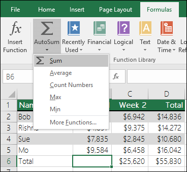
AutoSum creates the formula for you, so that you don’t have to do the typing. However, if you prefer typing the formula yourself, see the SUM function.
Add based on conditions
-
Use the SUMIF function when you want to sum values with one condition. For example, when you need to add up the total sales of a certain product.
-
Use the SUMIFS function when you want to sum values with more than one condition. For instance, you might want to add up the total sales of a certain product, within a certain sales region.
Add or subtract dates
For an overview of how to add or subtract dates, see Add or subtract dates. For more complex date calculations, see Date and time functions.
Add or subtract time
For an overview of how to add or subtract time, see Add or subtract time. For other time calculations, see Date and time functions.
Need more help?
You can always ask an expert in the Excel Tech Community or get support in the Answers community.
Need more help?
Want more options?
Explore subscription benefits, browse training courses, learn how to secure your device, and more.
Communities help you ask and answer questions, give feedback, and hear from experts with rich knowledge.
See all How-To Articles
This tutorial demonstrates how to add values to cells and columns in Excel and Google Sheets.
Add Values to Multiple Cells
- To add a value to a range of cells, click on the cell where you want to display the result, and enter = (equal) and the cell reference of the first number then + (plus) and the number you want to add.
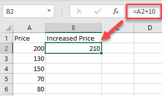
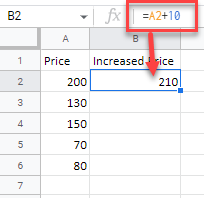
For this example, start with cell A2 (200). Cell B2 will show the Price in A2 increased by 10. So, in cell B2, enter:
=A2+10
As a result, the value in cell B2 is now 210 (value from A2 plus 10).
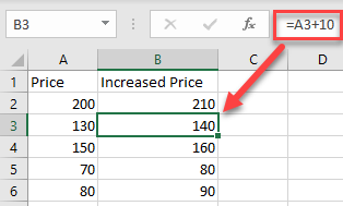
- Now copy this formula down the column to the rows below. Click on the cell where you entered the formula (F2) and place your cursor on the bottom right corner of the cell.
- When it changes to a plus sign, drag it down to the rest of the rows where you want to apply the formula (here, B2:B6).
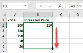
As a result of relative cell referencing, the constant (here, 10) remains the same, but the cell address changes according to the row you are in (so B3=A3+10, and so on).
Add Multiple Cells With Paste Special
You can also add a number to multiple cells and return the result as a number in the same cell.
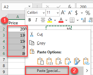
- First, select the cell with the value you want to add (here, cell C2), right-click, and from the drop-down menu, choose Copy (or use the shortcut CTRL + C).
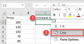
- After that, select the cells where you want to subtract the value and right-click on the data range (here, A2:A6). In the drop-down menu, click on Paste Special.
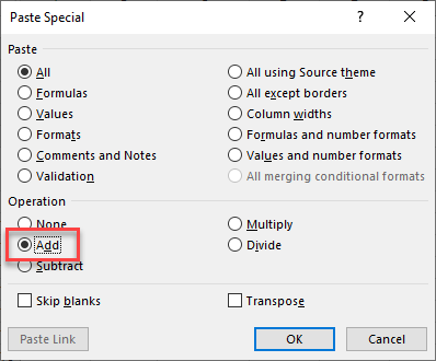
- The Paste Special window will appear. Under the Operation section choose Add, and then click OK.
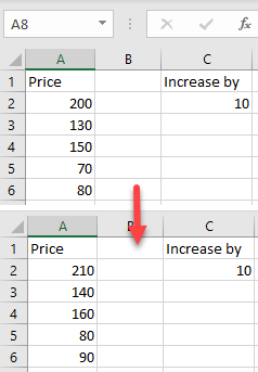
You’ll see the result as a number within the same cells. (In this example, 10 was added to each value from the data range A2:A6.) This method is better if you don’t want to display the results in a new column and don’t need to retain a record of the original values.
Add Column With Cell References
To add an entire column to another using cell references, select the cell where you want to display the result, and enter = (equal) and the cell reference for the first number then + (plus) and the reference for the cell you want to add.
For this example, calculate the summary of Price 1 (A2) and Price 2 (B2). So, in cell C2, enter:
=A2+B2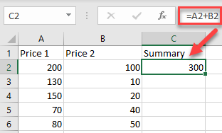
To apply the formula to an entire column, just copy the formula down to the rest of the rows in the table (here, C2:C6).
Now, you have a new column with the summary.
Using the methods above, you can also subtract, multiply, or divide cells and columns in Excel.
Add Cells and Columns in Google Sheets
In Google Sheets, you can add multiple cells using formulas in exactly the same ways as in Excel; except, you can’t use Paste Special.
Содержание
- Ways to add values in a spreadsheet
- Add based on conditions
- Add or subtract dates
- Add or subtract time
- Need more help?
- How to Add Values to Cells / Columns in Excel & Google Sheets
- Add Values to Multiple Cells
- Add Multiple Cells With Paste Special
- Add Column With Cell References
- Add Cells and Columns in Google Sheets
- SUM function
- Need more help?
- How to add text or character to every cell in Excel
- Excel formulas to add text/character to cell
- Concatenation operator
- CONCATENATE function
- CONCAT function
- How to add text to the beginning of cells
- How to add text to the end of cells in Excel
- Add characters to beginning and end of a string
- Combine text from two or more cells
- How to add special character to cell in Excel
- How to add text to formula in Excel
- How to insert text after Nth character
- How to add text before/after a specific character
- Add text after specific character
- Insert text before specific character
- How to add space between text in Excel cell
- How to add the same text to existing cells with VBA
- Prepend text to beginning
- Append text to end
- Add text or character to multiple cells with Ultimate Suite
Ways to add values in a spreadsheet
One quick and easy way to add values in Excel is to use AutoSum. Just select an empty cell directly below a column of data. Then on the Formula tab, click AutoSum > Sum. Excel will automatically sense the range to be summed. (AutoSum can also work horizontally if you select an empty cell to the right of the cells to be summed.)
AutoSum creates the formula for you, so that you don’t have to do the typing. However, if you prefer typing the formula yourself, see the SUM function.
Add based on conditions
Use the SUMIF function when you want to sum values with one condition. For example, when you need to add up the total sales of a certain product.
Use the SUMIFS function when you want to sum values with more than one condition. For instance, you might want to add up the total sales of a certain product, within a certain sales region.
Add or subtract dates
For an overview of how to add or subtract dates, see Add or subtract dates. For more complex date calculations, see Date and time functions.
Add or subtract time
For an overview of how to add or subtract time, see Add or subtract time. For other time calculations, see Date and time functions.
Need more help?
You can always ask an expert in the Excel Tech Community or get support in the Answers community.
Источник
How to Add Values to Cells / Columns in Excel & Google Sheets
This tutorial demonstrates how to add values to cells and columns in Excel and Google Sheets.
Add Values to Multiple Cells
- To add a value to a range of cells, click on the cell where you want to display the result, and enter = (equal) and the cell reference of the first number then + (plus) and the number you want to add.
For this example, start with cell A2 (200). Cell B2 will show the Price in A2 increased by 10. So, in cell B2, enter:
As a result, the value in cell B2 is now 210 (value from A2 plus 10).
- Now copy this formula down the column to the rows below. Click on the cell where you entered the formula (F2) and place your cursor on the bottom right corner of the cell.
- When it changes to a plus sign, drag it down to the rest of the rows where you want to apply the formula (here, B2:B6).
As a result of relative cell referencing, the constant (here, 10) remains the same, but the cell address changes according to the row you are in (so B3=A3+10, and so on).
Add Multiple Cells With Paste Special
You can also add a number to multiple cells and return the result as a number in the same cell.
- First, select the cell with the value you want to add (here, cell C2), right-click, and from the drop-down menu, choose Copy (or use the shortcut CTRL + C).
- After that, select the cells where you want to subtract the value and right-click on the data range (here, A2:A6). In the drop-down menu, click on Paste Special.
- The Paste Special window will appear. Under the Operation section choose Add, and then click OK.
You’ll see the result as a number within the same cells. (In this example, 10 was added to each value from the data range A2:A6.) This method is better if you don’t want to display the results in a new column and don’t need to retain a record of the original values.
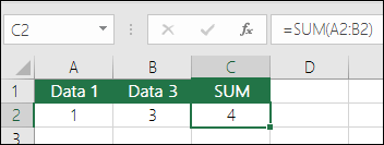
Add Column With Cell References
To add an entire column to another using cell references, select the cell where you want to display the result, and enter = (equal) and the cell reference for the first number then + (plus) and the reference for the cell you want to add.
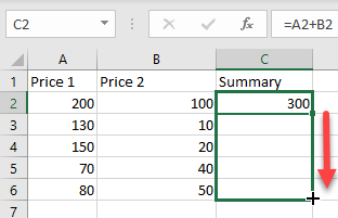
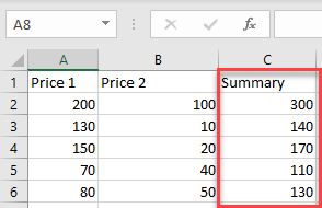
For this example, calculate the summary of Price 1 (A2) and Price 2 (B2). So, in cell C2, enter:
To apply the formula to an entire column, just copy the formula down to the rest of the rows in the table (here, C2:C6).
Now, you have a new column with the summary.
Using the methods above, you can also subtract, multiply, or divide cells and columns in Excel.
Add Cells and Columns in Google Sheets
In Google Sheets, you can add multiple cells using formulas in exactly the same ways as in Excel; except, you can’t use Paste Special.
Источник
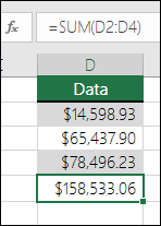
SUM function
The SUM function adds values. You can add individual values, cell references or ranges or a mix of all three.
=SUM(A2:A10) Adds the values in cells A2:10.
=SUM(A2:A10, C2:C10) Adds the values in cells A2:10, as well as cells C2:C10.

The first number you want to add. The number can be like 4, a cell reference like B6, or a cell range like B2:B8.
This is the second number you want to add. You can specify up to 255 numbers in this way.
This section will discuss some best practices for working with the SUM function. Much of this can be applied to working with other functions as well.
The =1+2 or =A+B Method – While you can enter =1+2+3 or =A1+B1+C2 and get fully accurate results, these methods are error prone for several reasons:
Typos – Imagine trying to enter more and/or much larger values like this:
Then try to validate that your entries are correct. It’s much easier to put these values in individual cells and use a SUM formula. In addition, you can format the values when they’re in cells, making them much more readable then when they’re in a formula.
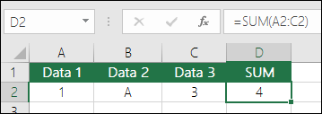
#VALUE! errors from referencing text instead of numbers
If you use a formula like:
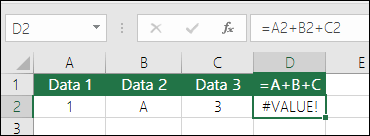
Your formula can break if there are any non-numeric (text) values in the referenced cells, which will return a #VALUE! error. SUM will ignore text values and give you the sum of just the numeric values.
#REF! error from deleting rows or columns
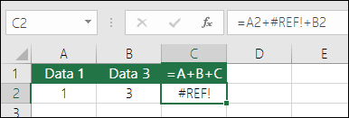
If you delete a row or column, the formula will not update to exclude the deleted row and it will return a #REF! error, where a SUM function will automatically update.
Formulas won’t update references when inserting rows or columns
If you insert a row or column, the formula will not update to include the added row, where a SUM function will automatically update (as long as you’re not outside of the range referenced in the formula). This is especially important if you expect your formula to update and it doesn’t, as it will leave you with incomplete results that you might not catch.
SUM with individual Cell References vs. Ranges
Using a formula like:
Is equally error prone when inserting or deleting rows within the referenced range for the same reasons. It’s much better to use individual ranges, like:
Which will update when adding or deleting rows.
I just want to Add/Subtract/Multiply/Divide numbers See this video series on Basic Math in Excel, or Use Excel as your calculator.
How do I show more/less decimal places? You can change your number format. Select the cell or range in question and use Ctrl+1 to bring up the Format Cells Dialog, then click the Number tab and select the format you want, making sure to indicate the number of decimal places you want.
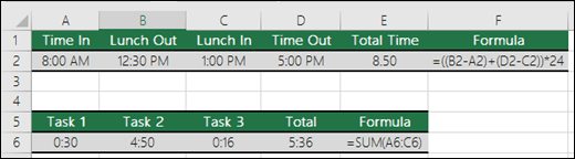
How do I add or subtract Times? You can add and subtract times in a few different ways. For example, to get the difference between 8:00 AM — 12:00 PM for payroll purposes you would use: =(«12:00 PM»-«8:00 AM»)*24, taking the end time minus the start time. Note that Excel calculates times as a fraction of a day, so you need to multiply by 24 to get the total hours. In the first example we’re using =((B2-A2)+(D2-C2))*24 to get the sum of hours from start to finish, less a lunch break (8.50 hours total).
If you’re simply adding hours and minutes and want to display that way, then you can sum and don’t need to multiply by 24, so in the second example we’re using =SUM(A6:C6) since we just need the total number of hours and minutes for assigned tasks (5:36, or 5 hours, 36 minutes).
For more information, see: Add or subtract time.
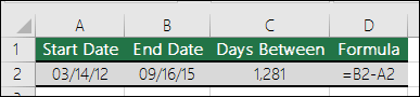
How do I get the difference between dates? As with times, you can add and subtract dates. Here’s a very common example of counting the number of days between two dates. It’s as simple as =B2-A2. The key to working with both Dates and Times is that you start with the End Date/Time and subtract the Start Date/Time.
How do I sum just visible cells? Sometimes, when you manually hide rows or use AutoFilter to display only certain data you also only want to sum the visible cells. You can use the SUBTOTAL function. If you’re using a total row in an Excel table, any function you select from the Total drop-down will automatically be entered as a subtotal. See more about how to Total the data in an Excel table.
Need more help?
You can always ask an expert in the Excel Tech Community or get support in the Answers community.
Источник
How to add text or character to every cell in Excel
 by Svetlana Cheusheva, updated on March 10, 2023
Wondering how to add text to an existing cell in Excel? In this article, you will learn a few really simple ways to insert characters in any position in a cell.
When working with text data in Excel, you may sometimes need to add the same text to existing cells to make things clearer. For example, you might want to put some prefix at the beginning of each cell, insert a special symbol at the end, or place certain text before a formula.
I guess everyone knows how to do this manually. This tutorial will teach you how to quickly add strings to multiple cells using formulas and automate the work with VBA or a special Add Text tool.
Excel formulas to add text/character to cell
To add a specific character or text to an Excel cell, simply concatenate a string and a cell reference by using one of the following methods.
Concatenation operator
The easiest way to add a text string to a cell is to use an ampersand character (&), which is the concatenation operator in Excel.
This works in all versions of Excel 2007 — Excel 365.
CONCATENATE function
The same result can be achieved with the help of the CONCATENATE function:
The function is available in Excel for Microsoft 365, Excel 2019 — 2007.
CONCAT function
To add text to cells in Excel 365, Excel 2019, and Excel Online, you can use the CONCAT function, which is a modern replacement of CONCATENATE:
Note. Please pay attention that, in all formulas, text should be enclosed in quotation marks.
These are the general approaches, and the below examples show how to apply them in practice.
How to add text to the beginning of cells
To add certain text or character to the beginning of a cell, here’s what you need to do:
- In the cell where you want to output the result, type the equals sign (=).
- Type the desired text inside the quotation marks.
- Type an ampersand symbol (&).
- Select the cell to which the text shall be added, and press Enter .
Alternatively, you can supply your text string and cell reference as input parameters to the CONCATENATE or CONCAT function.
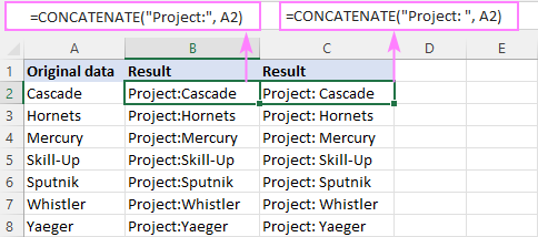
For example, to prepend the text «Project:» to a project name in A2, any of the below formulas will work.
In all Excel versions:
In Excel 365 and Excel 2019:
Enter the formula in B2, drag it down the column, and you will have the same text inserted in all cells.
Tip. The above formulas join two strings without spaces. To separate values with a whitespace, type a space character at the end of the prepended text (e.g. «Project: «).
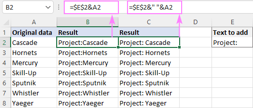
For convenience, you can input the target text in a predefined cell (E2) and add two text cells together:
Please notice that the address of the cell containing the prepended text is locked with the $ sign, so that it won’t shift when copying the formula down.
With this approach, you can easily change the added text in one place, without having to update every formula.
How to add text to the end of cells in Excel
To append text or specific character to an existing cell, make use of the concatenation method again. The difference is in the order of the concatenated values: a cell reference is followed by a text string.
For instance, to add the string «-US» to the end of cell A2, these are the formulas to use:
Alternatively, you can enter the text in some cell, and then join two cells with text together:
Please remember to use an absolute reference for the appended text ($D$2) for the formula to copy correctly across the column.

Add characters to beginning and end of a string
Knowing how to prepend and append text to an existing cell, there is nothing that would prevent you from using both techniques within one formula.
As an example, let’s add the string «Project:» to the beginning and «-US» to the end of the existing text in A2.
=CONCATENATE(«Project:», A2, «-US»)
=CONCAT(«Project:», A2, «-US»)
With the strings input in separate cells, this works equally well:

Combine text from two or more cells
To place values from multiple cells into one cell, concatenate the original cells by using the already familiar techniques: an ampersand symbol, CONCATENATE or CONCAT function.
For example, to combine values from columns A and B using a comma and a space («, «) for the delimiter, enter one of the below formulas in B2, and then drag it down the column.
Add text from two cells with an ampersand:
Combine text from two cells with CONCAT or CONCATENATE:
When adding text from two columns, be sure to use relative cell references (like A2), so they adjust correctly for each row where the formula is copied.

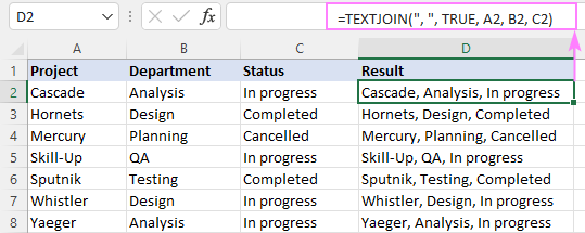
To combine text from multiple cells in Excel 365 and Excel 2019, you can leverage the TEXTJOIN function. Its syntax provides for a delimiter (the first argument), which makes the formular more compact and easier to manage.
For example, to add strings from three columns (A, B and C), separating the values with a comma and a space, the formula is:
=TEXTJOIN(«, «, TRUE, A2, B2, C2)
How to add special character to cell in Excel
To insert a special character in an Excel cell, you need to know its code in the ASCII system. Once the code is established, supply it to the CHAR function to return a corresponding character. The CHAR function accepts any number from 1 to 255. A list of printable character codes (values from 32 to 255) can be found here.
To add a special character to an existing value or a formula result, you can apply any concatenation method that you like best.
For example, to add the trademark symbol (в„ў) to text in A2, any of the following formulas will work:

How to add text to formula in Excel
To add a certain character or text to a formula result, just concatenate a string with the formula itself.
Let’s say, you are using this formula to return the current time:
=TEXT(NOW(), «h:mm AM/PM»)
To explain to your users what time that is, you can place some text before and/or after the formula.
Insert text before formula:
=»Current time: «&TEXT(NOW(), «h:mm AM/PM»)
=CONCATENATE(«Current time: «, TEXT(NOW(), «h:mm AM/PM»))
=CONCAT(«Current time: «, TEXT(NOW(), «h:mm AM/PM»))

Add text after formula:
=TEXT(NOW(), «h:mm AM/PM»)&» — current time»
=CONCATENATE(TEXT(NOW(), «h:mm AM/PM»), » — current time»)
=CONCAT(TEXT(NOW(), «h:mm AM/PM»), » — current time»)

Add text to formula on both sides:
=»It’s » &TEXT(NOW(), «h:mm AM/PM»)& » here in Gomel»
=CONCATENATE(«It’s «, TEXT(NOW(), «h:mm AM/PM»), » here in Gomel»)
=CONCAT(«It’s «, TEXT(NOW(), «h:mm AM/PM»), » here in Gomel»)

How to insert text after Nth character
To add a certain text or character at a certain position in a cell, you need to split the original string into two parts and place the text in between. Here’s how:
- Extract a substring preceding the inserted text with the help of the LEFT function:
LEFT(cell, n) - Extract a substring following the text using the combination of RIGHT and LEN:
RIGHT(cell, LEN(cell) -n) - Concatenate the two substrings and the text/character using an ampersand symbol.
The complete formula takes this form:
The same parts can be joined together by using the CONCATENATE or CONCAT function:
The task can also be accomplished by using the REPLACE function:
The trick is that the num_chars argument that defines how many characters to replace is set to 0, so the formula actually inserts text at the specified position in a cell without replacing anything. The position (start_num argument) is calculated using this expression: n+1. We add 1 to the position of the nth character because the text should be inserted after it.
For example, to insert a hyphen (-) after the 2 nd character in A2, the formula in B2 is:
=LEFT(A2, 2) &»-«& RIGHT(A2, LEN(A2) -2)
=CONCATENATE(LEFT(A2, 2), «-«, RIGHT(A2, LEN(A2) -2))
Drag the formula down, and you will have the same character inserted in all the cells:

How to add text before/after a specific character
To insert certain text before or after a particular character, you need to determine the position of that character in a string. This can be done with the help of the SEARCH function:
Once the position is determined, you can add a string exactly at that place by using the approaches discussed in the above example.
Add text after specific character
To insert some text after a given character, the generic formula is:
For instance, to insert the text (US) after a hyphen in A2, the formula is:
=LEFT(A2, SEARCH(«-«, A2)) &»(US)»& RIGHT(A2, LEN(A2) — SEARCH(«-«, A2))
=CONCATENATE(LEFT(A2, SEARCH(«-«, A2)), «(US)», RIGHT(A2, LEN(A2) -SEARCH(«-«, A2)))

Insert text before specific character
To add some text before a certain character, the formula is:
As you see, the formulas are very similar to those that insert text after a character. The difference is that we subtract 1 from the result of the first SEARCH to force the LEFT function to leave out the character after which the text is added. To the result of the second SEARCH, we add 1, so that the RIGHT function will fetch that character.
For example, to place the text (US) before a hyphen in A2, this is the formula to use:
=LEFT(A2, SEARCH(«-«, A2) -1) &»(US)»& RIGHT(A2, LEN(A2) -SEARCH(«-«, A2) +1)
=CONCATENATE(LEFT(A2, SEARCH(«-«, A2) -1), «(US)», RIGHT(A2, LEN(A2) -SEARCH(«-«, A2) +1))

- If the original cell contains multiple occurrences of a character, the text will be inserted before/after the first occurrence.
- The SEARCH function is case-insensitive and cannot distinguish lowercase and uppercase characters. If you aim to add text before/after a lowercase or uppercase letter, then use the case-sensitive FIND function to locate that letter.
How to add space between text in Excel cell
In fact, it is just a specific case of the two previous examples.
To add space at the same position in all cells, use the formula to insert text after nth character, where text is the space character (» «).
For example, to insert a space after the 10 th character in cells A2:A7, enter the below formula in B2 and drag it through B7:
=LEFT(A2, 10) &» «& RIGHT(A2, LEN(A2) -10)
=CONCATENATE(LEFT(A2, 10), » «, RIGHT(A2, LEN(A2) -10))
In all the original cells, the 10 th character is a colon (:), so a space is inserted exactly where we need it:

To insert space at a different position in each cell, adjust the formula that adds text before/after a specific character.
In the sample table below, a colon (:) is positioned after the project number, which may contain a variable number of characters. As we wish to add a space after the colon, we locate its position using the SEARCH function:
=LEFT(A2, SEARCH(«:», A2)) &» «& RIGHT(A2, LEN(A2)-SEARCH(«:», A2))
=CONCATENATE(LEFT(A2, SEARCH(«:», A2)), » «, RIGHT(A2, LEN(A2)-SEARCH(«:», A2)))

How to add the same text to existing cells with VBA
If you often need to insert the same text in multiple cells, you can automate the task with VBA.
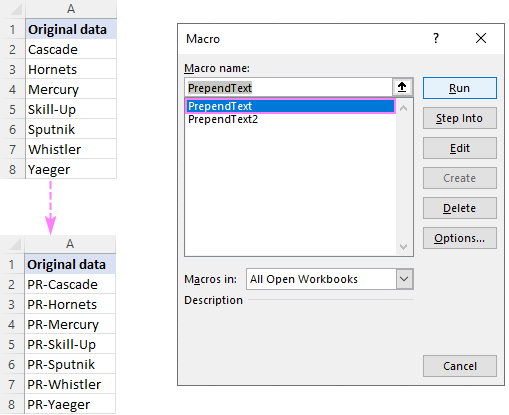
Prepend text to beginning
The below macros add text or a specific character to the beginning of all selected cells. Both codes rely on the same logic: check each cell in the selected range and if the cell is not empty, prepend the specified text. The difference is where the result is placed: the first code makes changes to the original data while the second one places the results in a column to the right of the selected range.
If you have little experience with VBA, this step-by-step guide will walk you through the process: How to insert and run VBA code in Excel.
Macro 1: adds text to the original cells
This code inserts the substring «PR-» to the left of an existing text. Before using the code in your worksheet, be sure to replace our sample text with the one you really need.
Macro 2: places the results in the adjacent column
Before running this macro, make sure there is an empty column to the right of the selected range, otherwise the existing data will be overwritten.

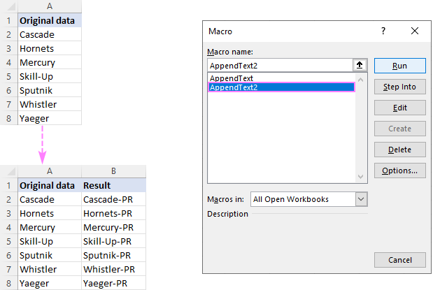
Append text to end
If you are looking to add a specific string/character to the end of all selected cells, these codes will help you get the work done quickly.
Macro 1: appends text to the original cells
Our sample code inserts the substring «-PR» to the right of an existing text. Naturally, you can change it to whatever text/character you need.

Macro 2: places the results in another column
This code places the results in a neighboring column. So, before you run it, make certain you have at least one empty column to the right of the selected range, otherwise your existing data will be overwritten.
Add text or character to multiple cells with Ultimate Suite
In the first part of this tutorial, you’ve learned a handful of different formulas to add text to Excel cells. Now, let’s me show you how to accomplish the task with a few clicks 🙂
With Ultimate Suite installed in your Excel, here are the steps to follow:
- Select your source data.
- On the Ablebits tab, in the Text group, click Add.
- On the Add Text pane, type the character/text you wish to add to the selected cells, and specify where it should be inserted:
- At the beginning
- At the end
- Before specific text/character
- After specific text/character
- After Nth character from the beginning or end
- Click the Add Text button. Done!
As an example, let’s insert the string «PR-» after the «-» character in cells A2:A7. For this, we configure the following settings:
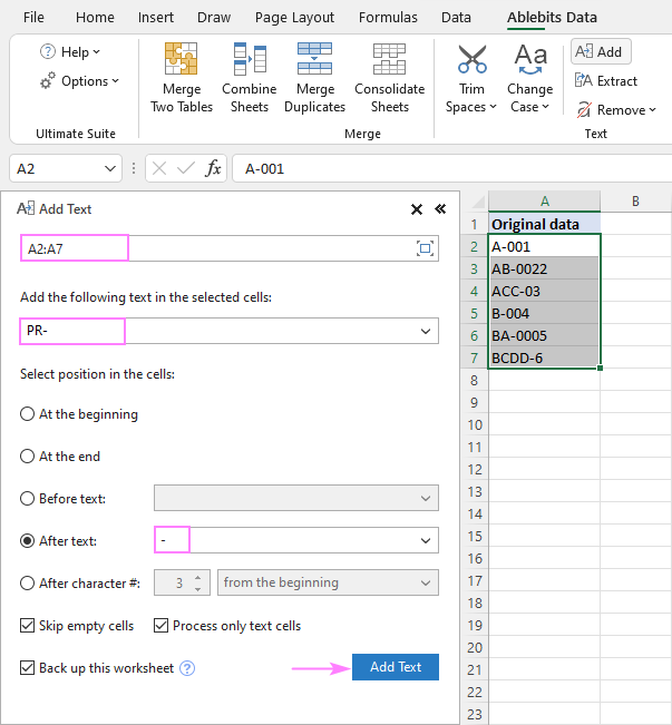
A moment later, we get the desired result:

These are the best ways to add characters and text strings in Excel. I thank you for reading and hope to see you on our blog next week!
Источник
![]()
Download Article
![]()
Download Article
Need to find the sum of a column, row, or set of numbers in Excel? Microsoft Excel comes with many mathematical functions, including multiple ways to add sets of numbers. This wikiHow article will teach you the easiest ways to add numbers, cell values, and ranges in Microsoft Excel.
-

1
Click the cell in which you want to display the sum.
-
2
Type an equal sign =. This indicates the beginning of a formula.
Advertisement
-
3
Type the first number you want to add. If you would rather add the value of an existing cell instead of typing a number manually, just click the cell you want to include in the equation. Otherwise, you can type a number manually.
- For example, if you click cell C3, the value of C3 will be the first number in your equation. If you type 1, the number 1 will be the first number in your equation.
-
4
Type a + sign.
-
5
Type another number select another cell. This adds the second number or value to your equation.
- You can add multiple cells or numbers at once if you’d like—just separate each number or address with another + sign.[1]
- For example, if you want to find the sum of cells C3, D4, and E5, your formula will look like this =C3+D4+E5.
- If you want to add 1 plus 1, your formula will look like this: =1+1 .
- You can add other operations, such as subtraction or multiplication, in the same equation. In this example, we’ll add the values of C3 and D4 and then subtract 2: =C3+D4-2
- You can add multiple cells or numbers at once if you’d like—just separate each number or address with another + sign.[1]
-
6
Press ↵ Enter or ⏎ Return. Now you’ll see the sum of the added numbers or values in the selected cell.


Advertisement
-
1
Click the cell in which you want to display the sum. The SUM function works like using the plus + sign, but is a bit easier to work with when you’re adding multiple cells and ranges.
-
2
Type an equal sign followed by the word SUM =SUM. This indicates the beginning of the SUM formula.
-
3
Type an opening parenthesis (. Your formula should now look like this: =SUM(.
-
4
Select the range of cells you want to add. Click and drag over all of the cells you want to add together. For example, if you want to add the values of all cells from A1 through A10, select all of those cells now.
- You can also select multiple columns and rows here. To select multiple non-adjacent columns and/or rows, hold down the Control key and as you select each range.
- You don’t have to select entire ranges with the SUM function—you can also enter individual numbers or cell addresses.
-
5
Type a clothing parenthesis ). This finishes the formula.
- Your formula should now look something like this: =SUM(B4,B8)
- In this example, we’ve selected cells B4 through B8
- If you selected non-adjacent ranges, each range will be separated by a comma. In this example, we selected B4 through C8 (two adjacent columns) and E4 through E5: =SUM(B4:C8,E4:E5)
- Your formula should now look something like this: =SUM(B4,B8)
-
6
Press ↵ Enter or ⏎ Return. The sum of the selected range now appears in this cell.


Advertisement
-
1
Click the cell immediately below or next to the values you want to add. AutoSum will automatically create a formula that adds the values of an adjacent column or row.[2]
- For example, if you want to add the values of cells A:2 through A:10, you would click cell A11.
- You can also add multiple columns or rows at the same time by selecting multiple cells. For example, to display the sums of values in columns A, B, and C, you could select cells A11, B11, and C11.
-
2
Click the AutoSum icon on the Home tab Σ. It’s the Sigma icon (which looks like an «E») on the Home tab at the top of Excel. A formula will then appear in the selected cell.
-
3
Press ↵ Enter or ⏎ Return. Now you’ll see the results of the formula in the cell.
- If you selected multiple blank cells, you’ll see each individual column or row’s value in the selected cells.


Advertisement
Ask a Question
200 characters left
Include your email address to get a message when this question is answered.
Submit
Advertisement
-
Use the SUMIF function to add cells that match certain criteria. For example, if you wanted to find the sum of all cells in A2 through A:10 that are greater than 1, you’d use =SUMIF(A2:A10, ">1").[3]
Thanks for submitting a tip for review!
Advertisement
About This Article
Article SummaryX
1. Use a plus sign to write out formulas like this: =4+5
2. Use the SUM formula to add values from one or more ranges.
3. Use AUTOSUM to automatically find the total of a column or row.
Did this summary help you?
Thanks to all authors for creating a page that has been read 108,680 times.
Is this article up to date?
Key Notes
- The value property can be used in both ways (you can read and write a value from a cell).
- You can refer to a cell using Cells and Range Object to set a cell value (to Get and Change also).
To set a cell value, you need to use the “Value” property, and then you need to define the value that you want to set. Here I have used some examples to help you understand this.
1. Enter a Value in a Cell
Let’s say you need to enter the value “Done” in cell A1. In that case, the code would be something like the below:
Range("A1").Value = "Done"
As you can see, I have first defined the cell address where I want to add the value, and then the value property. In the end, I have assigned the value “Done” using an equal “=” sign enclosed in double quotation marks.
You can also use the “Cells” property, just like the following code.
Cells(1, 1).Value = "Done"The above code also refers to cell A1.
Apart from this, there is one more way that you can use and that’s by not using the value property directly assigning the value to the cell.
Cells(1, 1) = "Done"But this is recommended to use the value property to enter a value in a cell.
Now let’s say you want to enter a number in a cell. In that case, you don’t need to use double quotation marks. You can write the code like the following.
Range("A1") = 99You can also DATE and NOW (VBA Functions) to enter a date or a timestamp in a cell using a VBA code.
Range("A1").Value = Date
Range("A2").Value = Now
And if you want to enter a value in the active cell then the code you need would be like:
ActiveCell.Value = Date2. Using an Input Box
If you want a user to specify a value to enter in a cell you can use an input box. Let’s say you want to enter the value in cell A1, the code would be like this:

Range("A1").Value = _
InputBox(Prompt:="Type the value you want enter in A1.")
In the above code, the value from cell A1 assigns to the value returned by the input box that returns the value entered by the user.
3. From Another Cell
You can also set cell value using the value from another cell. Let’s say if you want to add value to cell A1 from the cell B1, the code would be:
Range("A1") = Range("B1").Value
You can also refer to cell B1 without using the value property.
Range("A1") = Range("B1")4. Set Value in an Entire Range
Imagine you want to enter values in multiple cells or a range of cells instead of a single cell, in that case, you need to write code like the below:
Range("A1:A10").Value = Date
Range("B1, B10").Value = Now
In the first line of code, you have an entire range from cell A1 to A10, and in the second line, there are two cells B1 and B10.
Get Cell Value
As I said, you can use the same value property to get value from a cell.
1. Get Value from the ActiveCell
Let’s say you want to get the value from the active cell, in that case, you need to use the following code.
ActiveCell.Value = Range("A1")
In the above code, you have used the value property with the active cell and then assigned that value to cell A1.
2. Assign to a Variable
You can also get a value from a cell and further assign it to a variable.

Now in the above code, you have the variable “i” Which has the date as its data type. In the second line of the code, the value from cell A1 is assigned to the variable.
3. Show in a MsgBox
Now imagine, you want to show the value from cell A1 using a message box. In this case, the code would be like the below.
MsgBox Range("A1").Value
In the above code, the message box will take value from cell A1 and show it to the user.

Change Cell Value
You can also make changes to a cell value, and here I have shared a few examples that can help you to understand this.
1. Add a Number to an Existing Number
Let’s say if you want to add one to the number that you have in cell A1, you can use the following code.
Range("A1").Value = Range("A1").Value + 1The above code assigns value to cell A1 by taking value from cell A1 itself and adding one to it. But you can also use VBA IF THEN ELSE to write a condition to change only when there is a number in the cell.
If IsNumeric(Range("A1").Value) Then
  Range("A1").Value = Range("A1").Value + 1
End If
2. Remove First Character from Cell
Now, the following code removes the first character from the cell value and assigns the rest of the value back to the cell.
Range("A1").Value = Right(Range("A1").Value, Len(Range("A1").Value) - 1)More Tutorials
- Count Rows using VBA in Excel
- Excel VBA Font (Color, Size, Type, and Bold)
- Excel VBA Hide and Unhide a Column or a Row
- Excel VBA Range – Working with Range and Cells in VBA
- Apply Borders on a Cell using VBA in Excel
- Find Last Row, Column, and Cell using VBA in Excel
- Insert a Row using VBA in Excel
- Merge Cells in Excel using a VBA Code
- Select a Range/Cell using VBA in Excel
- SELECT ALL the Cells in a Worksheet using a VBA Code
- ActiveCell in VBA in Excel
- Special Cells Method in VBA in Excel
- UsedRange Property in VBA in Excel
- VBA AutoFit (Rows, Column, or the Entire Worksheet)
- VBA ClearContents (from a Cell, Range, or Entire Worksheet)
- VBA Copy Range to Another Sheet + Workbook
- VBA Enter Value in a Cell (Set, Get and Change)
- VBA Insert Column (Single and Multiple)
- VBA Named Range | (Static + from Selection + Dynamic)
- VBA Range Offset
- VBA Sort Range | (Descending, Multiple Columns, Sort Orientation
- VBA Wrap Text (Cell, Range, and Entire Worksheet)
- VBA Check IF a Cell is Empty + Multiple Cells
⇠ Back to What is VBA in Excel
Helpful Links – Developer Tab – Visual Basic Editor – Run a Macro – Personal Macro Workbook – Excel Macro Recorder – VBA Interview Questions – VBA Codes