
Excel for Microsoft 365 for Mac Excel 2021 for Mac Excel 2019 for Mac Excel 2016 for Mac Excel for Mac 2011 More…Less
Adding and subtracting in Excel is easy; you just have to create a simple formula to do it. Just remember that all formulas in Excel begin with an equal sign (=), and you can use the formula bar to create them.

Add two or more numbers in one cell
-
Click any blank cell, and then type an equal sign (=) to start a formula.
-
After the equal sign, type a few numbers separated by a plus sign (+).
For example, 50+10+5+3.
-
Press RETURN .
If you use the example numbers, the result is 68.
Notes:
-
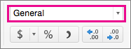
If you see a date instead of the result that you expected, select the cell, and then on the Home tab, select General.
-

-
Add numbers using cell references
A cell reference combines the column letter and row number, such as A1 or F345. When you use cell references in a formula instead of the cell value, you can change the value without having to change the formula.
-
Type a number, such as 5, in cell C1. Then type another number, such as 3, in D1.
-
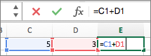
In cell E1, type an equal sign (=) to start the formula.
-
After the equal sign, type C1+D1.
-
Press RETURN .
If you use the example numbers, the result is 8.
Notes:
-
If you change the value of C1 or D1 and then press RETURN , the value of E1 will change, even though the formula did not.
-
If you see a date instead of the result that you expected, select the cell, and then on the Home tab, select General.
-
Get a quick total from a row or column
-
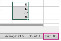
Type a few numbers in a column, or in a row, and then select the range of cells that you just filled.
-
On the status bar, look at the value next to Sum. The total is 86.
Subtract two or more numbers in a cell
-
Click any blank cell, and then type an equal sign (=) to start a formula.
-
After the equal sign, type a few numbers that are separated by a minus sign (-).
For example, 50-10-5-3.
-
Press RETURN .
If you use the example numbers, the result is 32.
Subtract numbers using cell references
A cell reference combines the column letter and row number, such as A1 or F345. When you use cell references in a formula instead of the cell value, you can change the value without having to change the formula.
-
Type a number in cells C1 and D1.
For example, a 5 and a 3.
-
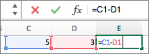
In cell E1, type an equal sign (=) to start the formula.
-
After the equal sign, type C1-D1.
-
Press RETURN .
If you used the example numbers, the result is 2.
Notes:
-
If you change the value of C1 or D1 and then press RETURN , the value of E1 will change, even though the formula did not.
-
If you see a date instead of the result that you expected, select the cell, and then on the Home tab, select General.
-
Add two or more numbers in one cell
-
Click any blank cell, and then type an equal sign (=) to start a formula.
-
After the equal sign, type a few numbers separated by a plus sign (+).
For example, 50+10+5+3.
-
Press RETURN .
If you use the example numbers, the result is 68.
Note: If you see a date instead of the result that you expected, select the cell, and then on the Home tab, under Number, click General on the pop-up menu.
Add numbers using cell references
A cell reference combines the column letter and row number, such as A1 or F345. When you use cell references in a formula instead of the cell value, you can change the value without having to change the formula.
-
Type a number, such as 5, in cell C1. Then type another number, such as 3, in D1.
-
In cell E1, type an equal sign (=) to start the formula.
-
After the equal sign, type C1+D1.
-
Press RETURN .
If you use the example numbers, the result is 8.
Notes:
-
If you change the value of C1 or D1 and then press RETURN , the value of E1 will change, even though the formula did not.
-
If you see a date instead of the result that you expected, select the cell, and then on the Home tab, under Number, click General on the pop-up menu.
-
Get a quick total from a row or column
-
Type a few numbers in a column, or in a row, and then select the range of cells that you just filled.
-
On the status bar, look at the value next to Sum=. The total is 86.
If you don’t see the status bar, on the View menu, click Status Bar.
Subtract two or more numbers in a cell
-
Click any blank cell, and then type an equal sign (=) to start a formula.
-
After the equal sign, type a few numbers that are separated by a minus sign (-).
For example, 50-10-5-3.
-
Press RETURN .
If you use the example numbers, the result is 32.
Subtract numbers using cell references
A cell reference combines the column letter and row number, such as A1 or F345. When you use cell references in a formula instead of the cell value, you can change the value without having to change the formula.
-
Type a number in cells C1 and D1.
For example, a 5 and a 3.
-
In cell E1, type an equal sign (=) to start the formula.
-
After the equal sign, type C1-D1.
-
Press RETURN .
If you used the example numbers, the result is -2.
Notes:
-
If you change the value of C1 or D1 and then press RETURN , the value of E1 will change, even though the formula did not.
-
If you see a date instead of the result that you expected, select the cell, and then on the Home tab, under Number, click General on the pop-up menu.
-
See also
Calculating operators and order of operations
Add or subtract dates
Subtract times
Need more help?
Want more options?
Explore subscription benefits, browse training courses, learn how to secure your device, and more.
Communities help you ask and answer questions, give feedback, and hear from experts with rich knowledge.

In this article, we will learn Different ways to add zeroes (0s) in front in Excel.
Scenario:
Adding Zero in front of the number in Excel. Default Excel doesn’t take zeros in front of the number in the cell. Have you ever tried to enter some data like 000123 into Excel? You’ll probably quickly notice Excel will automatically remove the leading zeros from the input number. This can be really annoying if you want those leading zeros in data and don’t know how to make Excel keep them. Fortunately there are quite a few ways to pad your numbers with zeros at the start. In this article, I’ll explain different ways to add or keep those leading zeros to your numbers.
Different functions to add zero (0) in front
As we know TEXT function is the most used function to add 0 in front but here I’ll explain more ways to add zeros (0s) to numbers.
- TEXT function
- RIGHT function
- BASE function
- Add 0 in pivot table values
Format as Text
One of the solutions is converting the format of the number to text because if we input 00xyz, excel considers this value as text and keeps its 0 in front. There are different ways to convert a number cell to text format.
- Using Custom format
- Using TEXT function
- Using Apostrophe ( ‘ ) in start of value while input
Custom Format
Let’s understand these methods one by one. Using a custom format to change the format is the easiest way to change the already existing numbers in range. Just select the range and Use shortcut Ctrl + 1 or select More number format from the drop down list on the Home tab showing General.
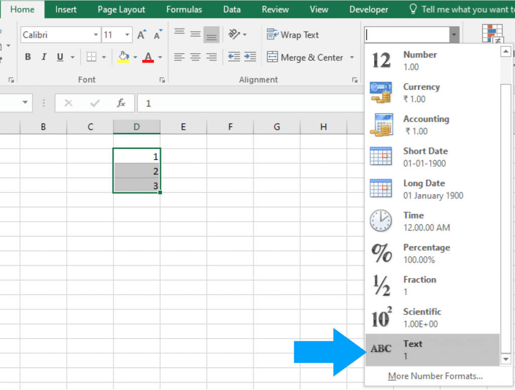
Change the format from General to Text.
- Select the range of cells you want to enter leading zeros in.
- Go to the Home tab.
- In the Numbers section click on the Format Dropdown selection.
- Choose Text from the format options.
Now if you try to enter numbers with leading zeros, they won’t disappear because they are entered as text values instead of numbers. Excel users can add a custom formatting to format numbers with leading zeros.
They will only appear to have leading zeros though. The underlying data won’t be changed into text with the added zeros.
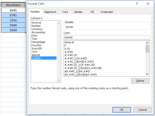
Add a custom format to show leading zeros.
- Select the range of cells you want to add leading zeros to and open up the Format Cells dialog box.
- Right click and choose Format Cells.
- Use the Ctrl + 1 keyboard shortcut.
- Go to the Number tab.
- Select Custom from the category options.
- Add a new custom format in the Type input. If you want the total number of digits including any leading zeros to be 6 then add 000000 as the custom format.
- Press the OK button.
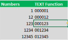
TEXT Function
The TEXT function will let you apply a custom formatting to any number data already in your spreadsheet.
= TEXT ( Value, Format)
- Value – This is the value you want to convert to text and apply formatting to.
- Format – This is the formatting to apply.

= TEXT ( B3, «000000» )
If you wanted to add zeros to a number in cell B3 so that the total number of digits is 6, then you can use the above formula.
Using Apostrophe ( ‘ ) in start
You can force Excel to enter a number as text by using a leading apostrophe.
This means you’ll be able to keep those zeros in front as you’re entering your data.
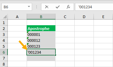
This method is quick and easy while entering data. Just type a ‘ character before any numbers. This will tell Excel the data is meant to be text and not a number.
When you press Enter, the leading zeros will stay visible in the worksheet. The ‘ will not be visible in the worksheet, but is still there and can be seen in the formula bar when the active cell cursor is on the cell.
RIGHT Function
Another way to get your zeros in front with a formula is using the RIGHT function. You can concatenate a string of zeros to the number and then slice off the extras using the RIGHT function.
The RIGHT function will extract the rightmost N characters from a text value.
= RIGHT ( Text, [Number])
- Text – This is the text you want to extract characters from.
- Number (Optional)- This is the number of characters to extract from the text. If this argument is not entered, then only the first character will be extracted.
= RIGHT ( «000000» & B3, 6 )
The above formula will concatenate several zeros to the start of a number in cell B3, then it will return the rightmost 6 characters resulting in some leading zeros.
BASE Function
You’ll notice this article describes 9 ways to add leading zeros, but my YouTube video only shows 8 ways.
That’s because I didn’t know you could use the BASE function to add leading zeros until someone mentioned it in the video comments.
The BASE function allows you to convert a number into a text representation with a given base.
The numbers you usually use are base 10, but you could use this function to convert a base 10 number into a base 2 (binary) representation.
= BASE ( Number, Base, [MinLength])
- Number – This is the number you want to convert to a text value in another base.
- Base – This is the base you want to convert the value to.
- MinLength (Optional) – This is the minimum length of the characters of the converted text value.
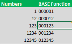
Use the formula
The above formula will convert a number in cell B3 into base 10 (it’s already a base 10 number but this will keep it as base 10) and convert it to a text value with at least 6 characters. If the converted value is less than 6 characters, it will pad the value with zeros to get a minimum of 6 characters.
Definitely a cool new use for a function I otherwise never use.
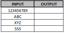
Add zero (0) only in front of numbers not on text values
Here we will consider the scenario which covers both text and numbers values in the same list. Now excel considers each cell different in terms of format. Now how to let excel know that if the cell has a number value then add 0 in front or else if the cell has text or any other value, then leave it as it is.
For this we will use a combination of two functions IF and ISNUMBER function. Here we have some values to try on.
The Generic formula goes on like
=IF(ISNUMBER(cell_ref),»0″&cell_ref, cell_ref)
Here
cell_ref : cell reference of the corresponding cell
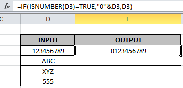
Use the formula in cell
=IF(ISNUMBER(F3),»0″&F3, F3)
Explanation: The ISNUMBER function checks the cell for number. IF function checks if the cell has a number then it adds zero in front of the number else it just returns the cell value.
As you can see in the above image the zero (0) is added in front of the number. Let’s check if this function works on other values. Copy the formula in other cells, select the cells taking the first cell where the formula is already applied, use shortcut key Ctrl+D
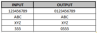
it will pad the value with zeros to get a minimum of one zero in front of characters. Definitely a cool new use for a function I otherwise never use.
Power Pivot Calculated Column
There is another option to add zeros into the pivot table. You can add them into a calculated column in Power Pivot. This way you can use the new column in the Filter, Rows or Column area of a pivot table.
= FORMAT ( Numbers[Number], «000000» )
In the Power Pivot add-in, you can add a new column and use the FORMAT function to create leading zeros in the column with a formula like above. A calculated column calculates a value for each row, so there is no need to wrap the function inside a cell. Now you can use this new column inside a pivot table’s Rows area just like any other column of data.
Summary
It can be frustrating to see all your zeros disappear when we don’t know why it’s happening or how to prevent it. As you can see, there are lots of ways to make sure all those zeros stick around in your data. Whatever your requirement, there is surely a good solution for you.
Here are all the observational notes using the formula in Excel
Notes :
- The formula can be used for both texts and numbers.
- The find and replace text should be sorted in a table. As we use indexes to find and replace, make sure that ‘find’ text has the same index as ‘replace’ text. It is better to have both lists side by side as we have in the second example.
- The generic formula has two SUBSTITUTE functions. You will need as many substitute functions as many you have replacements to do.
- wildcards help with extracting value from the substrings.
- The function supports logical operators like <, >, <>, = but these are used using double quote sign ( « ) with arguments. But if you are using cell reference for the criteria quotes can be ignored.
- Criteria argument should use quote sign («) for texts ( like «Gillen» ) or numbers ( like «>50» ).
Hope this article about Different ways to add zeroes (0s) in front in Excel is explanatory. Find more articles on calculating values and related Excel formulas here. If you liked our blogs, share it with your friends on Facebook. And also you can follow us on Twitter and Facebook. We would love to hear from you, do let us know how we can improve, complement or innovate our work and make it better for you. Write to us at info@exceltip.com.
Related Articles :
Excel REPLACE vs SUBSTITUTE function: The REPLACE and SUBSTITUTE functions are the most misunderstood functions. To find and replace a given text we use the SUBSTITUTE function. Where REPLACE is used to replace a number of characters in string.
Replace text from end of a string starting from variable position: To replace text from the end of the string, we use the REPLACE function. The REPLACE function use the position of text in the string to replace.
How to Check if a string contains one of many texts in Excel: To check if a string contains any of multiple texts, we use this formula. We use the SUM function to sum up all the matches and then perform a logic to check if the string contains any of the multiple strings.
Count Cells that contain specific text: A simple COUNTIF function will do the magic. To count the number of multiple cells that contain a given string we use the wildcard operator with the COUNTIF function.
Popular Articles :
50 Excel Shortcuts to Increase Your Productivity : Get faster at your tasks in Excel. These shortcuts will help you increase your work efficiency in Excel.
How to use the VLOOKUP Function in Excel : This is one of the most used and popular functions of excel that is used to lookup value from different ranges and sheets.
How to use the IF Function in Excel : The IF statement in Excel checks the condition and returns a specific value if the condition is TRUE or returns another specific value if FALSE.
How to use the SUMIF Function in Excel : This is another dashboard essential function. This helps you sum up values on specific conditions.
How to use the COUNTIF Function in Excel : Count values with conditions using this amazing function. You don’t need to filter your data to count specific values. Countif function is essential to prepare your dashboard.
There are many methods to do that, but I’ll go with the simple and quick methods to do it.
Method 1:
You can use Excel formula to do to calculate inside the cells, you just need to click on a cell and type = then do the calculation and press Enter.
Example : =1+1
(This will show the sum of 1+1)
The problem with this method, is that you’ll have to edit the cell each time you want to decrease or increase the numbers. For instance, let’s say we have 25 beers in stock, and we wasted 5 of them, then the formal will be written like this =25-5 to get the result of 20, and another day we wasted 2 beers, so we’ll go back to the cell and edit the formula to be like this =25-5-2 OR =25-7 and when we press Enter, it’ll be shown 18.. you do this process all over again each time you want to edit the results, and this method is the simplest one.
Method 2:
Excel uses cell references, and cell references is an indicator of which cell is selected. For example, if we say that we need to select the second cell of the second row, then that means and indicator to cell B2. Because the columns were sorted by alphabetical letters, and the rows sorted by numbers, so B2 means column #2 at row #2. That how cell references works. In fact, we can use cell references with variables numbers better than Method 1.
To use this method, you need to combine Method 1 with this method and only replace the numbers with the cells references.
Example : =A1+A2
In the previous example, it’ll show the sum of the cell#1 and cell#2 that are under column A, so whatever number in those two cells, will be added together and show the final result into the cell that you wrote the formula in. This method it’ll give you what you need without any extra work.
I’ve prepared a sample excel file that will be a good demonstration using Method 2 to start with, so you’ll know how it works.
Download
Product IDs, serial numbers and other reference numbers require a unique identifier to avoid confusion when referencing a product or specific data point. Although you can manually enter unique numbers for each item, doing so is tedious and time intensive for long lists. Instead, continuously increment a number in Microsoft Excel to produce these unique identifiers.
Formula Method
-
The most obvious way to increment a number in Excel is to add a value to it. Start with any value in cell A1, and enter «=A1+1» in cell A2 to increment the starting value by one. Copy the formula in A2 down the rest of the column to continuously increment the preceding number. This creates a long list of unique identifiers. You may use any number to increment the value, such as altering the formula to «=A1+567,» to create a less obvious pattern.
Increment Feature
-
Microsoft Excel inherently offers a numbering system to automatically create a series of incremented numbers. Enter any starting value in cell A1. Enter the next value in cell A2 to establish a pattern. Select those two cells and drag the bottom fill handle down the column to create a series of incremental numbers. As an example, entering 12 and 24 in cells A1 and A2 would create the series 12, 24, 36, 48, 60 when copied down to cell A5.
Sorting Incremental Numbers
-
If you need to sort data, opt for Excel’s incremental feature. The formula method works great. However, if you change the order of the cells, the formulas change as well. In contrast, Excel’s increment feature avoids formulas and enters the actual incremented value in the each cell. These numbers do not change, even if you reorder the list.
Paste Values
-
If you don’t want formula-incremented values to change, replace the formulas with the values they create. Select the cells you want to make constant and copy them. Right-click the selected cells and press «V» on your keyboard to replace the formulas with the actual, constant values.
Watch Video – 7 Quick and Easy Ways to Number Rows in Excel
When working with Excel, there are some small tasks that need to be done quite often. Knowing the ‘right way’ can save you a great deal of time.
One such simple (yet often needed) task is to number the rows of a dataset in Excel (also called the serial numbers in a dataset).
Now if you’re thinking that one of the ways is to simply enter these serial number manually, well – you’re right!
But that’s not the best way to do it.
Imagine having hundreds or thousands of rows for which you need to enter the row number. It would be tedious – and completely unnecessary.
There are many ways to number rows in Excel, and in this tutorial, I am going to share some of the ways that I recommend and often use.
Of course, there would be more, and I will be waiting – with a coffee – in the comments area to hear from you about it.
How to Number Rows in Excel
The best way to number the rows in Excel would depend on the kind of data set that you have.
For example, you may have a continuous data set that starts from row 1, or a dataset that start from a different row. Or, you might have a dataset that has a few blank rows in it, and you only want to number the rows that are filled.
You can choose any one of the methods that work based on your dataset.
1] Using Fill Handle
Fill handle identifies a pattern from a few filled cells and can easily be used to quickly fill the entire column.
Suppose you have a dataset as shown below:

Here are the steps to quickly number the rows using the fill handle:
Note that Fill Handle automatically identifies the pattern and fill the remaining cells with that pattern. In this case, the pattern was that the numbers were getting incrementing by 1.
In case you have a blank row in the dataset, fill handle would only work till the last contiguous non-blank row.
Also, note that in case you don’t have data in the adjacent column, double-clicking the fill handle would not work. You can, however, place the cursor on the fill handle, hold the right mouse key and drag down. It will fill the cells covered by the cursor dragging.
2] Using Fill Series
While Fill Handle is a quick way to number rows in Excel, Fill Series gives you a lot more control over how the numbers are entered.
Suppose you have a dataset as shown below:
Here are the steps to use Fill Series to number rows in Excel:
This will instantly number the rows from 1 to 26.
Using ‘Fill Series’ can be useful when you’re starting by entering the row numbers. Unlike Fill Handle, it doesn’t require the adjacent columns to be filled already.
Even if you have nothing on the worksheet, Fill Series would still work.
Note: In case you have blank rows in the middle of the dataset, Fill Series would still fill the number for that row.
3] Using the ROW Function
You can also use Excel functions to number the rows in Excel.
In the Fill Handle and Fill Series methods above, the serial number inserted is a static value. This means that if you move the row (or cut and paste it somewhere else in the dataset), the row numbering will not change accordingly.
This shortcoming can be tackled using formulas in Excel.
You can use the ROW function to get the row numbering in Excel.
To get the row numbering using the ROW function, enter the following formula in the first cell and copy for all the other cells:
=ROW()-1
The ROW() function gives the row number of the current row. So I have subtracted 1 from it as I started from the second row onwards. If your data starts from the 5th row, you need to use the formula =ROW()-4.
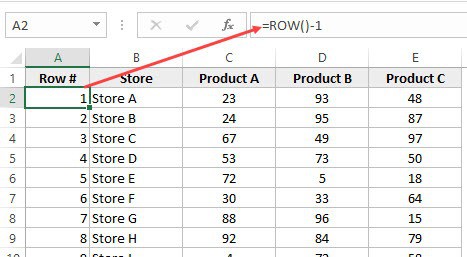
The best part about using the ROW function is that it will not screw up the numberings if you delete a row in your dataset.
Since the ROW function is not referencing any cell, it will automatically (or should I say AutoMagically) adjust to give you the correct row number. Something as shown below:

Note that as soon as I delete a row, the row numbers automatically update.
Again, this would not take into account any blank records in the dataset. In case you have blank rows, it will still show the row number.
You can use the following formula to hide the row number for blank rows, but it would still not adjust the row numbers (such that the next row number is assigned to the next filled row).
IF(ISBLANK(B2),"",ROW()-1)
4] Using the COUNTA Function
If you want to number rows in a way that only the ones that are filled get a serial number, then this method is the way to go.
It uses the COUNTA function that counts the number of cells in a range that are not empty.
Suppose you have a dataset as shown below:
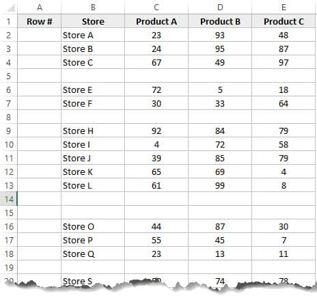
Note that there are blank rows in the above-shown dataset.
Here is the formula that will number the rows without numbering the blank rows.
=IF(ISBLANK(B2),"",COUNTA($B$2:B2))
The IF function checks whether the adjacent cell in column B is empty or not. If it’s empty, it returns a blank, but if it’s not, it returns the count of all the filled cells till that cell.
5] Using SUBTOTAL For Filtered Data
Sometimes, you may have a huge dataset, where you want to filter the data and then copy and paste the filtered data into a separate sheet.
If you use any of the methods shown above so far, you will notice that the row numbers remain the same. This means that when you copy the filtered data, you will have to update the row numbering.
In such cases, the SUBTOTAL function can automatically update the row numbers. Even when you filter the data set, the row numbers will remain intact.
Let me show you exactly how it works with an example.
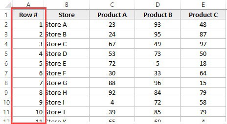
Suppose you have a dataset as shown below:

If I filter this data based on Product A sales, you will get something as shown below:

Note that the serial numbers in Column A are also filtered. So now, you only see the numbers for the rows that are visible.
While this is the expected behavior, in case you want to get a serial row numbering – so that you can simply copy and paste this data somewhere else – you can use the SUBTOTAL function.
Here is the SUBTOTAL function that will make sure that even the filtered data has continuous row numbering.
=SUBTOTAL(3,$B$2:B2)
The 3 in the SUBTOTAL function specifies using the COUNTA function. The second argument is the range on which COUNTA function is applied.
The benefit of the SUBTOTAL function is that it dynamically updates when you filter the data (as shown below):

Note that even when the data is filtered, the row numbering update and remains continuous.
6] Creating an Excel Table
Excel Table is a great tool that you must use when working with tabular data. It makes managing and using data a lot easier.
This is also my favorite method among all the techniques shown in this tutorial.
Let me first show you the right way to number the rows using an Excel Table:
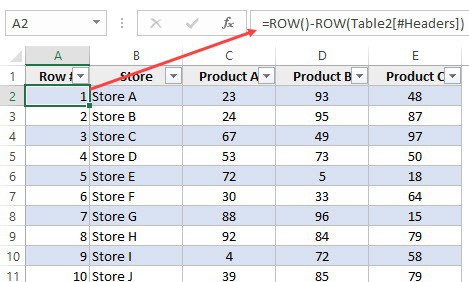
Note that in the formula above, I have used Table2, as that is the name of my Excel table. You can replace Table2 with the name of the table you have.
There are some added benefits of using an Excel Table while numbering rows in Excel:
- Since Excel Table automatically inserts the formula in the entire column, it works when you insert a new row in the Table. This means that when you insert/delete rows in an Excel Table, the row numbering would automatically update (as shown below).

- If you add more rows to the data, Excel Table would automatically expand to include this data as a part of the table. And since the formulas automatically update in the calculated columns, it would insert the row number for the newly inserted row (as shown below).


7] Adding 1 to the Previous Row Number
This is a simple method that works.
The idea is to add 1 to the previous row number (the number in the cell above). This will make sure that subsequent rows get a number that is incremented by 1.
Suppose you have a dataset as shown below:
Here are the steps to enter row numbers using this method:
- In the cell in the first row, enter 1 manually. In this case, it’s in cell A2.
- In cell A3, enter the formula, =A2+1
- Copy and paste the formula for all the cells in the column.

The above steps would enter serial numbers in all the cells in the column. In case there are any blank rows, this would still insert the row number for it.
Also note that in case you insert a new row, the row number would not update. In case you delete a row, all the cells below the deleted row would show a reference error.
These are some quick ways you can use to insert serial numbers in tabular data in Excel.
In case you are using any other method, do share it with me in the comments section.
You May Also Like the Following Excel Tutorials:
- Delete Blank Rows in Excel (with and without VBA).
- How to Insert Multiple Rows in Excel (4 Methods).
- How to Split Multiple Lines in a Cell into a Separate Cells / Columns.
- 7 Amazing Things Excel Text to Columns Can Do For You.
- Highlight EVERY Other ROW in Excel.
- How to Compare Two Columns in Excel.
- Insert New Columns in Excel