
Excel for Microsoft 365 Excel 2021 Excel 2019 Excel 2016 Excel 2013 Excel 2010 Excel 2007 More…Less
Excel can help you calculate the age of a person in different ways. The table below shows common methods to do so, using the Date and time functions.
To use these examples in Excel, drag to select the data in the table, then right-click the selection and pick Copy. Open a new worksheet, the right-click cell A1 and choose Paste Options > Keep Source Formatting.
|
Data |
|
|---|---|
|
10/2/2012 |
|
|
5/2/2014 |
|
|
6/3/2014 |
|
|
7/3/2014 |
|
|
6/3/2002 |
|
|
Formula |
Description |
|
=(YEAR(NOW())-YEAR(A2)) |
The result is the age of person—the difference between today and the birthdate in A2. This example uses the YEAR and NOW functions. If this cell doesn’t display a number, ensure that it is formatted as a number or General. Learn how to format a cell as a number or date. |
|
=YEAR(NOW())-1960 |
The age of a person born in 1960, without using cell references. If this cell doesn’t display as a number, ensure that it is formatted as a number or General. Learn how to format a cell as a number or date. |
|
=YEARFRAC(A3,A5) |
Calculates the year-fractional age between the dates in A5 and A3. |
|
=(A5-A6)/365.25 |
Calculates the age between the dates in A5 and A6, which is 12.08. To account for a leap year occurring every 4 years, 365.25 is used in the formula. |
|
=(«10/2/2014»-«5/2/2014») |
Calculates the number of days between two dates without using cell references, which is 153. |
|
=DAYS(TODAY(),»2/15/79″) |
The number of days between two dates, using two date functions. The two arguments of the DAYS function can be actual dates, cell references, or another date and time function—such as the TODAY function. |
|
=(YEAR(NOW())-YEAR(A3))*12+MONTH(NOW())-MONTH(A3) |
The number of months between A3 and the current date. This example uses the YEAR function , NOW function, and MONTH function. If this cell doesn’t display as a number, ensure that it is formatted as a number or General. Learn how to format a cell as a number or date. |
|
=NETWORKDAYS(A3,A2,A3:A5) |
The number of whole working days between the two dates in A2 and A3, which is 107. Working days exclude weekends and holidays. The last argument, A3:A5, lists the holidays to be subtracted from the working days. This example uses the NETWORKDAYS function. |
|
=DAYS360(A2,A3,TRUE) |
The number of days between the two dates in A2 and A3, which is 570. This is based on a 360-day year (twelve 30-day months) that are typical in accounting calculations. This example uses the DAYS360 function. |
|
=EDATE(A3,-4) |
Convert this to a date format and this should be 1/2/2014, which is four months (or -4) prior to the date in A3. This example uses the EDATE function, which is used to calculate maturity dates on banking notes. |
Related
-
Learn about all Date and Time functions.
-
Learn more about Detect errors in formulas.
-
Learn how to calculate the difference between dates using functions from Google Sheets: DATEDIF, DAYS360, and EDATE.
Need more help?
Top Methods to Calculate Age in Excel
In Excel, one can calculate the exact age of a person using different techniques. Age can be calculated in years, months, days, hours, and so on. For calculating the age, the beginning and ending dates need to be specified. Besides age, one can calculate the duration of a project, the time gap between two specific dates, the years of existence of an organization, etc.
For example, one can calculate the number of days between 01/16/2018 (in cell A1) and 01/30/2018 (in cell B1). The formula “=DATEDIF(A1,B1,“d”)” returns 14 days. Type the formula without the starting and ending double quotation marks.
Calculating the time period is easy if the start and end dates represent the beginning and the ending of a month respectively. However, in cases where this is not true, the complexities associated with the calculations increase. In such cases, Excel can prove to be of help.
The purpose of calculating the age is to study the period of survival of a person, event, project, corporate, and so on. It must be noted that Excel does not have a specific function for calculating age. But, different formulas of Excel can be used for the same.
Table of contents
- Top Methods to Calculate Age in Excel
- How to Calculate Age in Excel?
- Example #1–DATEDIF to Calculate Age in Completed Years
- Example #2–YEARFRAC to Calculate Age in Fractional Years
- Example #3–DATEDIF and Arithmetic Operations to Calculate Age in Completed and Fractional Months
- Example #4–DATEDIF to Calculate Age in Days
- Example #5–CONCATENATE and DATEDIF to Calculate Age in Years, Months, and Days
- Calculate Age Using VBA
- The Cautions While Calculating Age in Excel
- Frequently Asked Questions
- Recommended Articles
- How to Calculate Age in Excel?
How to Calculate Age in Excel?
Let us consider some examples to understand the calculation of age in Excel.
You can download this Calculate Age Excel Template here – Calculate Age Excel Template
Example #1–DATEDIF to Calculate Age in Completed Years
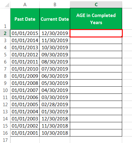
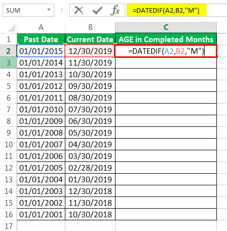
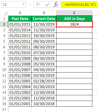
The following image shows two dates in each row. We want to calculate the time gap between the past date (column A) and the current date (column B).
Use the DATEDIF excel functionDATEDIf is a date function that finds the difference between two dates, which can now be expressed in years, months, or days. This function’s syntax is =DATEDIF (Start Date, End Date, Unit).read more to calculate the time gap (age) in completed years.
The steps to calculate the age in years by using the DATEDIF excel function are listed as follows:
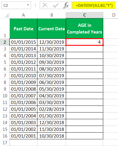
- Enter the following formula in cell C2.
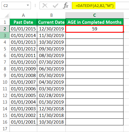
- Press the “Enter” key. The output appears in cell C2, as shown in the following image. Hence, for the dates specified in row 2, the completed years of age are 4.

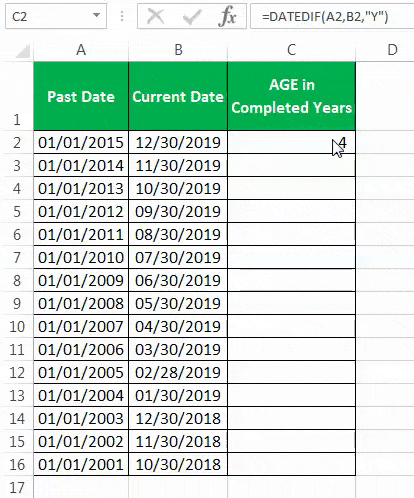
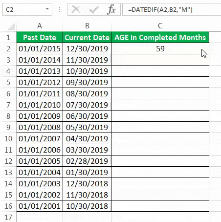
- Drag the DATEDIF formula of cell C2 till cell C16. The outputs appear for the entire dataset. This is shown in the following image.

Description of the DATEDIF function: The syntax of the DATEDIF function is, “DATEDIF(start_date,end_date,unit).” The function accepts the following mandatory arguments:
- Start date: This is the beginning date of the given period. In this example, it is the past date.
- End date: This is the last date of the given period. In this example, it is the current date.
- Unit: This returns the time gap between the two dates in different units. These units are years, months, and days. It can take any of the following six values:
- For “unit” equal to “y,” “m,” or “d,” the completed number of years, months or days is calculated respectively.
- For “unit” equal to “md,” “yd,” or “ym,” the days (ignoring years and months), days (ignoring years) or months (ignoring days and years) are calculated respectively.
Explanation: The DATEDIF function (entered in step 1) returns the completed years of age between any two specified dates. This is because we have set the “unit” argument at “y,” which represents years. For row 2, the completed years between 01/01/2015 and 12/30/2019 are 4.
Note: In the DATEDIF formula, the end date should always be greater than the start date. If not, Excel returns the “#NUM!” error. The DATEDIF function works in almost all versions of Excel.
However, Excel does not help while entering the arguments of the DATEDIF function, unlike in the case of the other functions. This is because the DATEDIF is a hidden function, which is not available in the Formulas tab of Excel.
Example #2–YEARFRAC to Calculate Age in Fractional Years
Working on the data of example #1, let us calculate the time gap (age) in fractions of years with the help of the YEARFRAC excel functionYEARFRAC Excel is a built-in Excel function that is used to get the year difference between two date infractions. This function returns the difference between two dates infractions like 1.5 Years, 1.25 Years, 1.75 Years, etc. So using this function we can find the year difference between two dates accurately.read more.
The steps for the same are listed as follows:
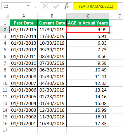
Step 1: Enter the following formula in cell C2.
“=YEARFRAC(A2,B2,1)”
Note: For the syntax of the YEARFRAC function, refer to the “description of the YEARFRAC function” given at the end of this example.
Step 2: Press the “Enter” key. Next, drag the preceding formula to the remaining cells of column C. The outputs of column C are shown in the following image.
Description of YEARFRAC function: The syntax of the YEARFRAC function is “YEARFRAC(start_date,end_date,[basis]).” The function accepts the following arguments:
- Start date: This represents the starting date (past date) of the given period.
- End date: This represents the ending date (current date) of the given period.
- Basis: This is the basis on which the number of days is counted while calculating the fractional years. It can take any of the following five values:
- For “basis” equal to 0 or 4, [(30 days per month)/(360 days per year)] is calculated as per the US or the European conventions respectively.
- For “basis” equal to 1, 2 or 3, [(actual days)/(actual days in the year)], [(actual days)/360] or [(actual days)/365] is calculated respectively.
The “start date” and “end date” are mandatory arguments, while “basis” is an optional argument. If the “basis” argument is omitted, Excel assumes the basis as 0.
Explanation: For row 2, the gap (in years) between 01/01/2015 and 01/01/2019 is 4. The remaining gap between 01/02/2019 and 12/30/2019 is calculated in fractions. The actual days in this period are 365-2=363. The two days that have been excluded are 01/01/2019 and 12/31/2019.
Since the basis is entered as 1, the actual days within the period are divided by the actual days within the year. Hence, 363/365=0.994521. So, the YEARFRAC function returns 4+0.99=4.99 for row 2. Likewise, the fractional years for the remaining rows are calculated by Excel.
Example #3–DATEDIF and Arithmetic Operations to Calculate Age in Completed and Fractional Months
Working on the data of example #1, we want to perform the following tasks:
- Calculate the time gap (age or period) between two dates in completed months.
- Calculate the time gap (age or period) between two dates in fractional months.
For task “a,” use the DATEDIF function of Excel. For task “b,” use the subtraction and division operations.
a. The steps for calculating the age (time gap) in completed months by using the DATEDIF excel function are listed as follows:
Step 1: Enter the following formula in cell C2.
“=DATEDIF(A2,B2,“M”)”
Step 2: Press the “Enter” key. The output is 59, as shown in the following image.
Step 3: Drag the DATEDIF formula till cell C16, as shown in the following image. The outputs appear in column C.
Explanation: The DATEDIF formula, entered in step 1, calculates the time gap in completed months. This is because the “m” entered in this formula corresponds to months.
For row 2, the number of completed months between 01/01/2015 and 12/30/2019 is 59. This includes 48 months of the four years (2015-2018, both inclusive) plus 11 months of the final year (2019).
The month of December 2019 has been excluded from the calculation as it is not a completed month. In this way, the number of completed months for the remaining rows has been calculated by Excel.
b. The steps for calculating the age in excel (time gap) in fractional months are listed as follows:
Step 1: Enter the following formula in cell C2.
“=+(B2-A2)/30”
Note: The formula “=(B2-A2)/30” returns the same output as the formula “=+(B2-A2)/30.” Hence, one can ignore the “plus” sign of the preceding formula.
Step 2: Press the “Enter” key. Then, drag the formula of cell C2 till cell C16. The outputs are shown in the following image.

Explanation: For row 2, Excel calculates the completed months as 59. The remaining days are divided by 30 and added to this number in decimals. To make it simpler, the total days between 01/01/2015 and 12/30/2019 are divided by 30.
So, 1824/30=60.8. Hence, the total fractional months for the second row are calculated as 60.8. Likewise, the fractional months for the remaining rows are computed by Excel.
Note: For more details on how we obtained the total days as 1824 (for row 2), refer to example #4.
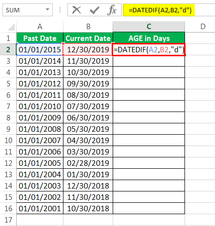
Example #4–DATEDIF to Calculate Age in Days
Working on the data of example #1, we want to calculate the age (time gap) in excel in number of days. Use the DATEDIF function of Excel.
The steps for the same are listed as follows:
Step 1: Enter the following DATEDIF formula in cell C2.
“=DATEDIF(A2,B2,“d”)”
Step 2: Press the “Enter” key. The output in cell C2 is 1824, as shown in the following image.
Step 3: Drag the formula of cell C2 till cell C16. The dragging process and the resulting outputs are shown in the following image.
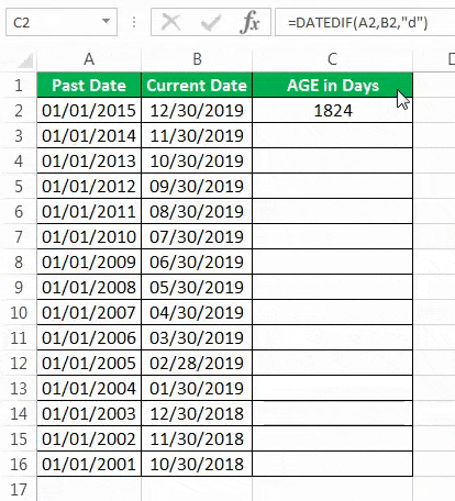
Explanation: For each row, Excel has calculated the number of days between the starting and the ending dates. This is because we entered “d” in the DATEDIF formula, which corresponds to days.
Example #5–CONCATENATE and DATEDIF to Calculate Age in Years, Months, and Days
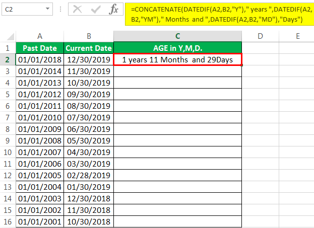
Working on the data of example #1, we want to calculate the age in excel (time gap) between two dates in years, months, and days. Notice that a new date has been entered in cell A2.
Use the CONCATENATEThe CONCATENATE function in Excel helps the user concatenate or join two or more cell values which may be in the form of characters, strings or numbers.read more and the DATEDIF functions of Excel.
The steps for the given task are listed as follows:
Step 1: Enter the following formula in cell C2.
“=CONCATENATE(DATEDIF(A2,B2,”Y”),” years “,DATEDIF(A2,B2,”YM”),” Months and “,DATEDIF(A2,B2,”MD”),”Days”)”

Step 2: Press the “Enter” key. The output in cell C2 is “1 years 11 months and 29 days.”
Step 3: Drag the formula to the remaining cells of column C. The outputs are shown in the following image.
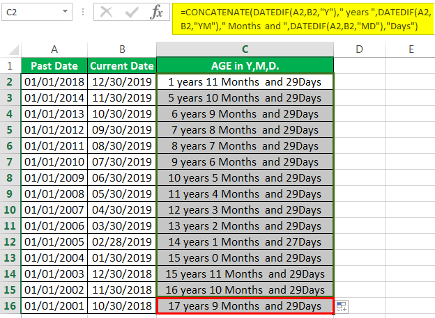
Explanation: In the formula entered in step 1, we have concatenated (joined) three DATEDIF formulas with the help of the CONCATENATE function. Moreover, the text strings “years,” “months,” and “days” are entered after each DATEDIF formula. This implies that in the final output, the result of each DATEDIF formula will be joined with the respective text strings.
The following notations have been used in the formula (in step 1):
- “Y”: This calculates the completed years between the two specified dates.
- “YM”: This calculates the number of months over and above the completed years.
- “MD”: This calculates the number of days over and above the completed months.
For row 2, the number of completed years is 1, which is counted from 01/01/2018 to 01/01/2019. The number of completed months is counted from 01/01/2019 to 12/01/2019, which equals 11. Finally, the number of days is counted from 12/01/2019 to 12/30/2019, which equals 29.
Hence, the output is 1 year, 11 months, and 29 days.
Calculate Age Using VBA
Let us calculate the time gap (age) using excel VBA. The steps for the same are listed as follows:
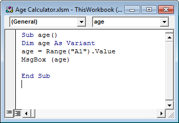
Step 1: Open the VBA editorThe Visual Basic for Applications Editor is a scripting interface. These scripts are primarily responsible for the creation and execution of macros in Microsoft software.read more by pressing the keys “Alt+F11” together.
Step 2: Define the code, as shown in the following image. We have defined “age” as a variant whose source has been given as cell A1 of the worksheet.
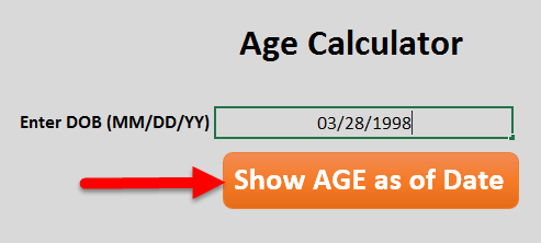
Step 3: In the age calculator, enter the date in the mm/dd/yyyy format.
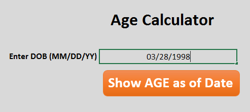
Step 4: Click the button “show age as of date.”
Step 5: The output is shown in the following image.

Explanation: The system has calculated the age from 03/28/1998 to 01/16/2019. Hence, the output is 20 years, 9 months, and 19 days.
The Cautions While Calculating Age in Excel
The cautions governing the calculation of age in Excel are listed as follows:
- Ensure that two dates are necessarily specified for calculating the age in excel. From these two dates, one must precede the other. While applying the DATEDIF function, remember that the end date exceeds the start date.
- Confirm that the two dates specified are recognized by Excel as valid dates. If not, Excel returns the “#VALUE!” error. If dates appear as text, convert them to dates by using the “format cells” option of Excel.
- Make sure that the two dates entered are in the same format. For instance, both dates can be in the format mm/dd/yyyy.
Note: Excel stores the dates as consecutive numbers having a difference of 1. The reason for storing dates as serial numbers (like 43466) is to facilitate calculations. However, to understand such serial numbers, it is essential to format them as dates.
Frequently Asked Questions
1. What does it mean to calculate age in Excel?
In Excel, one can calculate the age beginning from a certain date. Likewise, the time gap between two dates or the time taken to complete a project can be calculated.
For calculating such time periods, one must ensure that the beginning and the ending dates specified are recognized by Excel as valid dates. Thereafter, the calculations can be performed in Excel. To calculate age between two given dates, one can use the DATEDIF or YEARFRAC functions of Excel.
Note: For the syntax of the DATEDIF and YEARFRAC functions, refer to the examples of this article.
2. How to calculate the age from the date of birth in Excel?
Let us calculate the age from a random date of birth, 10/25/2002 (in cell A1), till the current date (11/25/2021). The steps are listed as follows:
a. Enter the formula “=INT((TODAY()-A1)/365)” in any cell, say B1. Exclude the beginning and ending double quotation marks while entering the formula.
b. Press the “Enter” key.
The output 19 appears in cell B1. The INT function rounds the decimal number downwards to the nearest integer. Had we entered the formula as “=(TODAY()-A1)/365,” we would have obtained 19.098.
The TODAY function returns the current date. The difference between the current date and the date in cell A1 is carried out. The resulting output is in days. This is divided by 365 to obtain the age in number of years.
Note: The output of the formula (entered in step “a”) updates automatically to reflect the change in the current date.
3. How to calculate the age in years and months in Excel?
Let us calculate the age between 06/14/1996 (in cell A1) and the current date (11/25/2021) in years and months. The steps are listed as follows:
a. Enter the formula [=DATEDIF(A1,TODAY(),”y”)&” years, “&DATEDIF(A1,TODAY(),”ym”)& ” months “] in any cell, say C1. Exclude the beginning and ending square brackets while entering the formula.
b. Press the “Enter” key.
The output in cell C1 is “25 years, 5 months.” This is obtained without the double quotation marks but with the spaces and the comma between the numbers and the text strings.
Notice that, in the formula, we entered a space preceding and succeeding the words “years” and “months.” We also inserted a comma following the word “years.” Consequently, spaces and a comma are inserted at the respective places in the output. A space after “months” may or may not be entered in the formula.
Note: The TODAY function updates on its own each time the workbook is opened. Hence, the current date updates automatically and so does the output of the formula (entered in step a).
Recommended Articles
This has been a guide to calculating age in Excel. Here we discuss how to calculate age in an Excel sheet using the DATEDIF formula, CONCATENATE formula, and Excel VBA code along with practical examples and a downloadable template. You may learn more about Excel from the following articles –
- Concatenate in VBAIn VBA, concatenation refers to joining two values or strings together with the «&» symbol (ampersand operator). We must include spaces when using the & operator, else VBA will interpret it as long.read more
- Calculation of Excel Formula for Grade
- Custom Format of Numbers in ExcelExcel custom number formatting is nothing but making the data look better or visually appealing. Excel has many inbuilt number formatting. On top of this, we can customize the Excel number formatting by changing the format of the numbers.read more
- Insert Row Keyboard Shortcut in ExcelThe insertion of an excel row is simply the addition of a new (blank) row to the worksheet. The insertion of a row is eased with the help of shortcuts.read more
- Excel Create ListA list can be created in Excel to define a list of items/values as predefined values. It may be created using the Data Validation tool so that users may select from a list rather than entering their own values.read more
To calculate the age of a person in Excel, use DATEDIF and TODAY. The DATEDIF function has three arguments.
1. Enter the date of birth into cell A2.

2. Enter the TODAY function into cell B2 to return today’s date.

3. The DATEDIF function below calculates the age of a person.

Note: fill in «y» for the third argument to get the number of complete years between the date of birth and today’s date.
4. Calculate the age of a person without displaying today’s date.

5. Calculate the age of a person on a specific date.

Note: the DATE function accepts three arguments: year, month and day.
6. The age formula below calculates the age of a person in years, months and days.

Note: fill in «ym» for the third argument to ignore years and get the number of months between two dates. Fill in «md» for the third argument to ignore months and get the number of days between two dates. Use the & operator to join strings.
Watch Video – How to Calculate Age in Excel (in Years, Months, and Days)
Using a combination of Excel functions and the date of birth, you can easily calculate age in Excel. You can either calculate the age till the current date or between the specified period of time.
The technique shown here can also be used in other situations such as calculating the duration of a project or the tenure of the service.
How to Calculate Age in Excel
In this tutorial, you’ll learn how to calculate age in Excel in:
- The number of years elapsed till the specified date.
- The number of Years, Months, and Days elapsed till the specified date.
You can also download the Excel Age Calculator Template.
Calculate Age in Excel – Years Only
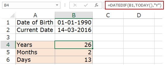
Suppose you have the date of birth in cell B1, and you want to calculate how many years have elapsed since that date, here is the formula that’ll give you the result:
=DATEDIF(B1,TODAY(),"Y")

If you have the current date (or the end date) in a cell, you can use the reference instead of the TODAY function. For example, if you have the current date in cell B2, you can use the formula:
=DATEDIF(B1,B2,"Y")
DATEDIF function is provided for the compatibility with Lotus 1-2-3.
One of the things that you’ll notice when you use this function is that there is no IntelliSense available for this function. No tooltip appears when you use this function.
This means that while you can use this function in Excel, you need to know the syntax and how many arguments this function takes.
If you’re interested in knowing more about DATEDIF function, read the content of the box below. If not, you can skip this and move to the next section.
Syntax of DATEDIF function:
=DATEDIF(start_date, end_date, unit)
It takes 3 arguments:
- start_date: It’s a date that represents the starting date value of the period. It can be entered as text strings in double-quotes, as serial numbers, or as a result of some other function, such as DATE().
- end_date: It’s a date that represents the end date value of the period. It can be entered as text strings in double-quotes, as serial numbers, or as a result of some other function, such as DATE().
- unit: This would determine what type of result you get from this function. There are six different output that you can get from the DATEDIF function, based on what unit you use. Here are the units that you can use:
- “Y” – returns the number of completed years in the specified time period.
- “M” – returns the number of completed months in the specified time period.
- “D” – returns the number of completed days in the specified period.
- “MD” – returns the number of days in the period, but doesn’t count the ones in the Years and Months that have been completed.
- “YM” – returns the number of months in the period, but doesn’t count the ones in the years that have been completed.
- “YD” – returns the number of days in the period, but doesn’t count the ones in the years that have been completed.
You can also use the YEARFRAC function to calculate the age in Excel (in years) in the specified date range.
Here is the formula:
=INT(YEARFRAC(B1,TODAY()))

The YEARFRAC function returns the number of years between the two specified dates and then the INT function returns only the integer part of the value.
NOTE: It’s a good practice to use the DATE function to get the date value. It avoids any erroneous results that may occur when entering the date as text or any other format (which is not an acceptable date format).
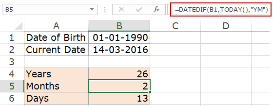
Calculate Age in Excel – Years, Months, & Days
Suppose you have the date of birth in cell A1, here are the formulas:
To get the year value:
=DATEDIF(B1,TODAY(),"Y")
To get the month value:
=DATEDIF(B1,TODAY(),"YM")
To get the day value:
=DATEDIF(B1,TODAY(),"MD")
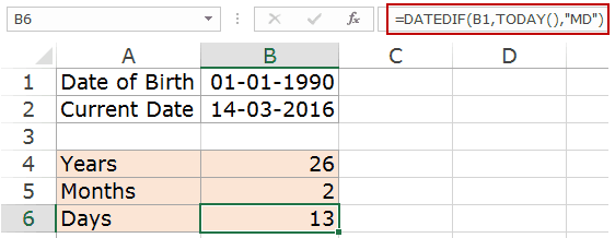
Now that you know how to calculate the years, months and days, you can combine these three to get a text that says 26 Years, 2 Months, and 13 Days. Here is the formula that will get this done:
=DATEDIF(B1,TODAY(),"Y")&" Years "&DATEDIF(B1,TODAY(),"YM")&" Months "&DATEDIF(B1,TODAY(),"MD")&" Days"

Note that the TODAY function is volatile and its value would change every day whenever you open the workbook or there is a change in it. If you want to keep the result as is, convert the formula result to a static value.
Download the Excel Age Calculator Template

Excel Functions Used:
Here is a list of functions used in this tutorial:
- DATEDIF() – This function calculates the number of days, months, and years between two specified dates.
- TODAY() – It gives the current date value.
- YEARFRAC() – It takes the start date and the end date and gives you the number of years that have passed between the two dates. For example, if someone’s date of birth is 01-01-1990, and the current date is 15-06-2016, the formula would return 26.455. Here the integer part represents the number of years completed, and the decimal part represents additional days that have passed after 26 years.
- DATE() – It returns the date value when you specify the Year, Month, and Day value arguments.
- INT() – This returns the integer part of a value.
You May Also Like the Following Excel Tutorials:
- Free Excel Holiday Calendar Template.
- Calculating Working Days between Two Dates in Excel.
- Excel Calendar Template.
- How to Automatically Insert Date and Time Stamp in Excel.
- Calculate Months Between Two Dates in Excel
- How to SUM values between two dates in Excel
- Get Day Name from Date in Excel
Excel doesn’t have a dedicated function for calculating age, but there are several ways we can use someone’s date of birth to compute the person’s age. We won’t just learn how to compute someone’s age in years, we’ll even boil their age down to months and days.
There are several formulas, as well as combinations of formulas, that we can use to calculate age in excel. We’ll talk about each of those formulas one by one. So without further ado, let’s jump in.
 1")
Recommended Reading: How to Calculate Years of Service in Excel
Calculating Age in Excel With the DATEDIF function
The DATEDIF function does exactly what the name suggests. It calculates the DATE+DIF (where DIF may be inferred as DIFFERENCE) and gives us the output in our preferred unit. For instance, let’s say David’s DOB is 10/01/1990.
We want to know how old David is today.
 2")
So, we’ll use the following formula to calculate David’s age:
=DATEDIF(A2, TODAY(), "y") & " year(s)" //current age in years
=DATEDIF(A2, TODAY(), "m") & " month(s)" //current age in months
=DATEDIF(A2, TODAY(), "d") & " day(s)" //current age in days
The first argument is David’s DOB, the second argument is today’s date, and «y» tells the formula that we want the output in terms of years. Finally, we have concatenated a text «year(s)» which is displayed as an identifier against the age. So, as on the day of writing (Jun 24, 2021), Excel tells us that David is 30 years old.
Excel subtracted the serial number of the date entered in the first argument from the serial number of the date entered in the second argument to compute the difference in terms of days. Then, it converted it into years and eliminated the decimal value to give us the final output.
In the next row, we change «y» to «m» and the identifier from «year(s)» to «month(s)». This changes the formula so that it now gives us David’s age in the number of months, which is 368 months.
To compute the number of months, it does the same thing, except that the days are converted to months instead of years. We can even take this a step further and use «d» in the final argument to compute David’s age in the number of days. In this case, we do this in the third row, where our final output comes to 11,210 days.
Calculating Age as on a Given Date in the Past
We can also tweak the DATEDIF function slightly and calculate David’s age as on any specific date. For this, we’ll use the DATE function instead of the TODAY function and nest it in the DATEDIF function’s end_date argument.
Let’s assume that we want to calculate David’s age as of Christmas 2018.
 3")
We’ll use the following formula:
=DATEDIF(A2, DATE(2018,12,25), "y") & " year(s)" //past age in years
=DATEDIF(A2, DATE(2018,12,25), "m") & " month(s)" //past age in months
=DATEDIF(A2, DATE(2018,12,25), "d") & " day(s)" //past age in days
This formula works exactly the same way as the previous one. As you can see, the only difference is in the second argument where we have supplied a specific date instead of using the TODAY function.
The output, of course, is 28 years. This makes sense because the date we’ve entered is roughly 2.5 years in the past. Since the output ignores the value after the decimal, we get 28 (i.e., 30 – 2) years as our output. In the subsequent rows, we get 338 months as our output when we enter «m» in the final argument and 10,298 days as our output when we enter «d» in the final argument.
Calculating Age as on a Given Date in the Future
This exercise has inspired David’s curious side. He was hoping to get busy with some financial planning. He has set a few financial goals for himself and wishes to compute his age at a future date to compute his taxability and maturities for investments.
 4")
No worries, let’s help David figure out his age using the following formula:
=DATEDIF(A2, DATE(2045,12,25), "y") & " year(s)" //future age in years
=DATEDIF(A2, DATE(2045,12,25), "m") & " month(s)" //future age in months
=DATEDIF(A2, DATE(2045,12,25), "d") & " day(s)" //future age in days
This formula will help us compute David’s age in terms of years as on Christmas day of the year 2045. There’s no change in the formula except the year in the DATE function. Naturally, the formula returns David’s age as on the supplied date as 55 years. Changing the final argument to «m» gives us 662 months, and changing the final argument to «d» gives us 20,160 days.
Calculating Age in Years with the YEARFRAC function
Before we begin working on this, note that DATDIF is generally a more preferable way to compute age. It’s possible to compute age using the YEARFRAC function as well, but it allows us to compute the age only in terms of years.
 5")
To compute David’s age using the YEARFRAC function, we’ll use the following formula:
=INT(YEARFRAC(A2, TODAY()))
Let’s start with why we have the INT function in the formula. The INT function has a sole purpose – removing values after the decimal. When the YEARFRAC function returns, for example, 10.3 years and relays it to the INT function, it will convert it to 10 years.
Moving on, let’s see what the YEAFRAC function does. The first argument in the function is the start_date argument and the second argument is the end_date argument. It’s similar to what we saw with the DATEDIF function, except that there is no third argument and the YEARFRAC function’s output does contain a decimal value.
In our example, the YEARFRAC function returns 30.69 years. This output is relayed to the INT function, which gives us our final output of 30 years.
Recommended Reading: How to Add Years to a Date in Excel
Calculating Age in Years, Months, and Days
The previous formulas helped David calculate his age in terms of years, months, and days. However, what formula must he use to compute his exact age? For instance, in this format – 20 years, 6 months, 15 days.
 6")
We know that when we want to connect outputs of two formulas, we use a concatenation (&). Therefore, we’ll use the following formula:
=DATEDIF(A2,TODAY(),"y") &" year(s) " & DATEDIF(A2,TODAY(),"ym") &" month(s) " & DATEDIF(A2,TODAY(),"md") &" day(s) "
So, why use «ym» and «md» instead of «m» and «d» like we did before? Well, «ym» instructs the formula to compute the difference only between the months entered in the first and second argument. Similarly, «md» instructs the formula to compute the difference only in the days entered in the first and second argument.
In this case, these are the differences we want. Think about it—using «m» and «d» would have given us the total months/days between David’s DOB and today—and that’s not what we want.
Our output, therefore, is «30 year(s) 8 month(s) 9 day(s) «. We can format the text strings in the formula to add commas or spaces as required.
Calculating When a Person Will Turn X Years Old
David’s curiosity is driving him nuts. Lucky for us, he wants to learn everything there is about calculating ages in Excel. He now wants to figure out when he will turn 35 years, 45 years, and 55 years so he can plan his life accordingly.
 7")
More power to him, I say. Let’s help him with our next formula:
=DATE(YEAR(A2) + 35, MONTH(A2), DAY(A2)) //When David turns 35 years old
=DATE(YEAR(A3) + 45, MONTH(A2), DAY(A2)) //When David turns 45 years old
=DATE(YEAR(A2) + 55, MONTH(A2), DAY(A2)) //When David turns 55 years old
This is a pretty straightforward formula where we have used the DATE function to add 35 years to David’s DOB. The DATE argument picks up the year, month, and day component and compiles them into a valid Excel date.
In fact, if David’s date of birth were split into three different cells, each containing a different component of his DOB (i.e., year, month, and day), this formula would still work. We’d just need to reference the relevant cells instead of cell A2.
When the formula picks up the year component, we simply add 35 to it, which gives us our final output. In our example, David turns 35 on October 15, 2025, turns 45 on October 15, 2035, and turns 55 on October 15, 2045.
Calculating Age Difference Between Two Individuals
David is unstoppable but promises this will be his last exercise for computing ages. We are onboard. This time, David wants to see how he can compute the difference between the ages of two individuals. He has a list of DOBs he wants to compare his own age with.
 8")
To accomplish this, we’ll use the following formula:
=DATEDIF(A2,B2,"y") & " year(s)"
We know that any time we want to compute the difference in dates, we default to the DATEDIF function.
However, there is one small problem. When David wants to compare his age with someone younger than him, the DATEDIF function’s cell references will need to change. The date in the start_date argument must necessarily occur before the value in the end_date argument, otherwise, the function will return a #NUM error (like we can see in the C5 cell).
It can be fixed by referencing cell B2 in the first argument and A2 in the second argument. However, if you’re working with a large dataset, you may need a more convenient alternative; a formula you can drag down across the column.
To remedy this, let’s just use two very simple functions and plain algebra, like so:
 9")
=INT(ABS((A2-B2)/365)) &" year(s)"
Let’s start from what’s inside the inner-most brackets. The (A2-B2) is a subtraction of two dates. Excel will subtract the serial numbers of each date and the output will be the difference between these dates in terms of days. Next, we just divide it by 365 to convert it to years.
Then, we have the ABS function. The ABS function ensures that we always have a positive value. For instance, in the second row, the date in B3 falls after the date in A3, and that gives us a negative number. The ABS function will convert this value into a positive number and relay it to the INT function.
INT function, as we discussed before, gives us the integer value (i.e., removes the value after the decimal). This gives us a nice, clean output of 4 years, 4 years, and 6 years, respectively.
An important thing to note here is that you must always nest the ABS function inside the INT function and not vice versa. This is because the INT function rounds positive numbers towards zero, and negative numbers away from 0. For instance, in the second row, if we nest the INT function inside the ABS function, our output changes to 5.
This concludes our age calculating spree with David. We used a range of functions that can help us compute a person’s age, or even figure out when a person will turn x number of years. While you work on mastering these techniques, we’ll put together another tutorial for you. Until next time.