
Maintenance Alert: Saturday, April 15th, 7:00pm-9:00pm CT. During this time, the shopping cart and information requests will be unavailable.
Categories: Advanced Excel
Tags: Excel Range Formula
An essential skill any Excel user should know is how to determine the range of values in Excel. Most businesses don’t have time to waste sorting through rows and rows in Excel in order to find the highest and lowest values of revenue, sales, or other information. The difference between the highest and lowest figures in a group of data – the range – can be valuable in accurate decision making, budgeting, and forecasting.
Let’s pretend you are the purchasing manager for Revelation, Inc., a small business that distributes computers. You can bid bulk pricing for raw materials that will significantly improve Revelation’s profits. The sooner you can purchase materials, the better, because the price increases the closer they are to the ship date. You can use sales data from the prior fiscal year to budget for raw materials, and the range can help you forecast next year’s sales based on this year’s results. You can use the average sales per month for insight into what raw materials you should need when. Identifying that specific gap is also great for setting performance standards, because you can figure out how you perform against other months.
Because Excel offers multiple ways to write range formulas to suit your individual needs, here are three range formula options to get you started!
1. Minimum and Maximum Formulas
Revelation keeps a spreadsheet with information including the state, model, number of units, unit price, and total revenue for each product per state. The past year’s product sales are arranged as follows:
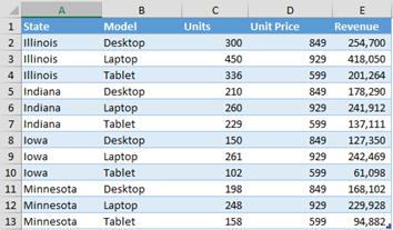
You need to find which products have the smallest and largest demand. This is a small list, but if you sell or resell a lot of product, the following formula can be invaluable. You can find minimum and maximum units easily with the MIN() and MAX() functions.
- In cell B15, type “=MIN(C2:C13)”.
- In cell B16, type “=MAX(C2:C13)”.
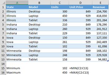
You now have a quick report of the fewest number of units sold in a state (102 tablets in Iowa) and the most sold (450 laptops in Illinois).
2. Top k and Bottom k Formulas
Suppose you’re interested in more data – not just the lowest selling item but the three lowest. You can find these with the SMALL() function. To use SMALL(), you’ll need two parameters:
- The same range or list of values as you used for MIN().
Note: If you are using multiple values instead of a single continuous range, you’ll need to place each set in parentheses.
- The value k, which is the desired position from the bottom of the list. If you’re looking for the smallest value, then k = 1. To find the second smallest value, k = 2, etc.
To find the largest three values, use the LARGE() function with the same parameters as SMALL().
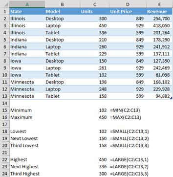
Note that SMALL() with k = 1 produces exactly the same result as MIN(). Similarly, LARGE() with k = 1 yields the same as MAX().
3. Conditional Minimum and Maximum Formulas
In some situations, you might need a minimum value that meets specific criteria. For example, you might want to know the fewest units sold for the spring quarter duration or for a specific product type.
Excel provides SUMIF(), COUNTIF(), and other helpful conditional formulas. Unfortunately, there is no MINIF() or MAXIF(), but you can create the same effect with a slightly more complicated method called an array formula. An array formula evaluates a range of cells instead of a single cell.
Typically an IF() formula tests the truth value of a single cell, but as an array formula, we can force it to evaluate each cell in a range. With an array formula you will get an error if you just press enter – #VALUE!. Remember to press CTRL, SHIFT, and ENTER after you finish your array formula.
Let’s find the minimum value for desktops. First, type the matching value (desktop) into the cell you compare your function to. If you are looking for desktop values, then type “desktop” in B18. The formula below will compare that cell reference to the range you are testing. Nest the MIN() and IF() statements as follows: “=MIN(IF(B2:B13=B18,C2:C13))” and press <CTRL>-<SHIFT>-<ENTER>.
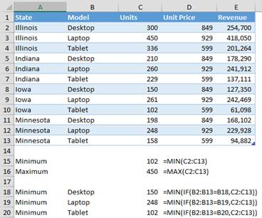
The three formulas in rows 18, 19, and 20 calculate the minimum numbers of desktops, laptops, and tablets sold. You can write identical formulas with MAX() to find the greatest number of each product sold.
Next Steps
Now you can use three different methods (Minimum and Maximum Formulas, Top k and Bottom k Formulas, Conditional Minimum and Maximum Formulas) to find the range of values in any data set.
PRYOR+ 7-DAYS OF FREE TRAINING
Courses in Customer Service, Excel, HR, Leadership,
OSHA and more. No credit card. No commitment. Individuals and teams.
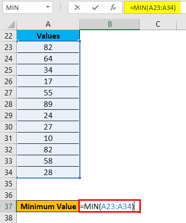
Range is the difference between minimum and maximum value in a dataset. In Excel you can calculate range using the functions MIN and MAX.
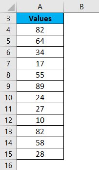
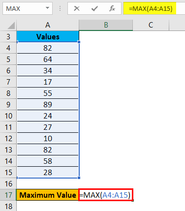
For example, if you have your data in cells A1 to A15, you can calculate range in a single formula:
=MAX(A1:15)-MIN(A1:A15)
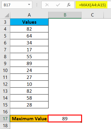
The first part of the formula, MAX(A1:A15), finds the highest value in the data (75 in the screenshot above).
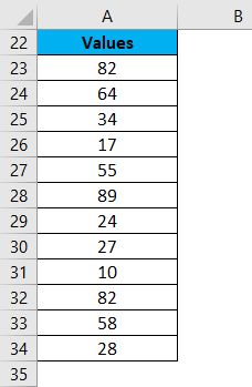
The second part, MIN(A1:15), finds the lowest value (14).
If you subtract the minimum from the maximum, you get range (61).
Calculating Range in Excel VBA
Range is so commonly needed, it is surprising there is no built-in RANGE function in Excel, which would make the calculation easier than the formula above. We could just use a formula like this:
=RANGE(A1:A15)Unfortunately, there is no built-in RANGE function in Excel.
However, with some basic VBA, we can create our own custom function that would work just like that.
Function Range(Data)
    ' Calculates range (maximum - minimum) of data

    Range = Application.WorksheetFunction.Max(Data) _
            - Application.WorksheetFunction.Min(Data)

End Function
With this function defined in VBA, we can now use it in a spreadsheet to calculate range more simply:
=RANGE(A1:A15)This gives the same result as
=MAX(A1:15)-MIN(A1:A15)
Note: Although «range» means a different, very common thing in Excel and VBA – a range of cells – it is not a reserved word in VBA and you can call your custom function RANGE. That said, you may want to consider another name to avoid any confusion, such as RNG.
Calculating Trading Range in Excel
In the financial markets, range is the difference between highest and lowest price (high and low) in a particular time period, such as a trading day. As above, it is calculated by subtracting the minimum (low) from the maximum (high):
Range = High – Low
If you have market data in the OHLC (open-high-low-close) format in Excel, simply take the cell containing the high and subtract the cell containing the low from it – see screenshot from ATR Calculator below.

Unlike most other market statistics and technical indicators, closing price does not enter the calculation of range in any way.
Calculating Range in ATR Calculator
You can calculate average range in the ATR Calculator by selecting «Range» in the drop-down box in cells K4/L4/M4. You can also see the range for each bar in column G.
Average True Range (ATR)
Average True Range (ATR) is a more advanced concept of range and more suitable in some types of markets. While the traditional (high minus low) range only considers the volatility (range) of the trading session itself, ATR also looks at overnight volatility (a possible price gap from the previous day’s close to the current day’s opening price).
Here you can see a detailed explanation of true range and ATR calculation.
Normally, when I use the word range in my tutorials about Excel, it’s a reference to a cell or a collection of cells in the worksheet.
But this tutorial is not about that range.
A ‘Range’ is also a mathematical term that refers to the range in a data set (i.e., the range between the minimum and the maximum value in a given dataset)
In this tutorial, I will show you really simple ways to calculate the range in Excel.
What is a Range?
In a given data set, the range of that data set would be the spread of values in that data set.
To give you a simple example, if you have a data set of student scores where the minimum score is 15 and the maximum score is 98, then the spread of this data set (also called the range of this data set) would be 73
Range = 98 – 15
‘Range’ is nothing but the difference between the maximum and the minimum value of that data set.
How to Calculate Range in Excel?
If you have a list of sorted values, you just have to subtract the first value from the last value (assuming that the sorting is in the ascending order).
But in most cases, you would have a random data set where it’s not already sorted.
Finding the range in such a data set is quite straightforward as well.
Excel has the functions to find out the maximum and the minimum value from a range (the MAX and the MIN function).
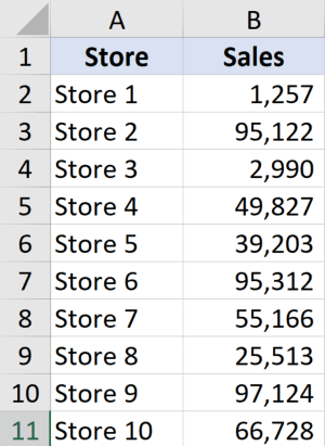
Suppose you have a data set as shown below, and you want to calculate the range for the data in column B.
Below is the formula to calculate the range for this data set:
=MAX(B2:B11)-MIN(B2:B11)
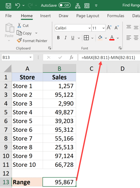
The above formula finds the maximum and the minimum value and gives us the difference.
Quite straightforward… isn’t it?
Calculate Conditional Range in Excel
In most practical cases, finding the range would not be as simple as just subtracting the minimum value from the maximum value
In real-life scenarios, you might also need to account for some conditions or outliers.
For example, you may have a data set where all the values are below 100, but there is one value that is above 500.
If you calculate arrange for this data set, it would lead to you making misleading interpretations of the data.
Thankfully, Excel has many conditional formulas that can help you sort out some of the anomalies.
Below I have a data set where I need to find the range for the sales values in column B.
If you look closely at this data, you would notice that there are two stores where the values are quite low (Store 1 and Store 3).
This could be because these are new stores or there were some external factors that impacted the sales for these specific stores.
While calculating the range for this data set, it might make sense to exclude these newer stores and only consider stores where there are substantial sales.
In this example, let’s say I want to ignore all those stores where the sales value is less than 20,000.
Below is the formula that would find the range with the condition:
=MAX(B2:B11)-MINIFS(B2:B11,B2:B11,">20000")
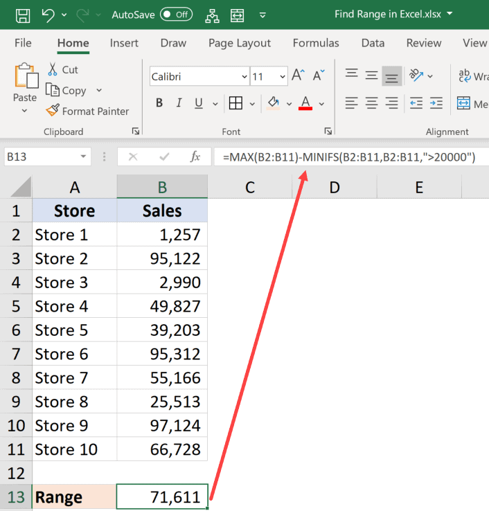
In the above formula, instead of using the MIN function, I have used the MINIFS function (it’s a new function in Excel 2019 and Microsoft 365).
This function finds the minimum value if the criteria mentioned in it are met. In the above formula, I specified the criteria to be any value that is more than 20,000.
So, the MINIFS function goes through the entire data set, but only considers those values that are more than 20,000 while calculating the minimum value.
This makes sure that values lower than 20,000 are ignored and the minimum value is always more than 20,000 (hence ignoring the outliers).
Note that the MINIFS is a new function in Excel is available only in Excel 2019 and Microsoft 365 subscription. If you’re using prior versions, you would not have this function (and can use the formula covered later in this tutorial)
If you don’t have the MINIF function in your Excel, use the below formula that uses a combination of IF function and MIN function to do the same:
=MAX(B2:B11)-MIN(IF(B2:B11>20000,B2:B11))
Just like I have used the conditional MINIFS function, you can also use the MAXIFS function if you want to avoid data points that are outliers in the other direction (i.e., a couple of large data points that can skew the data)
So, this is how you can quickly find the range in Excel using a couple of simple formulas.
I hope you found this tutorial useful.
Other Excel tutorials you may like:
- How to Calculate Standard Deviation in Excel
- How to Calculate Square Root in Excel
- How to Calculate and Format Percentages in Excel
Содержание
- How to Find Range in Excel (Easy Formulas)
- What is a Range?
- How to Calculate Range in Excel?
- Calculate Conditional Range in Excel
- Range in Excel
- Range in Excel
- How to Find Range in Excel?
- Range in Excel – Example #1
- Range in Excel – Example #2
- Range in Excel – Example #3
- Range in Excel – Example #4
- Things to Remember
- Recommended Articles
- Excel Function for Range
- Range Function in Excel
- Examples of Range Function in Excel
- Example #1 – Finding Maximum and Minimum
- Example #2 – How to Define and Use Ranges in Excel?
- Things to Remember
- Conclusion
- Recommended Articles
How to Find Range in Excel (Easy Formulas)
Normally, when I use the word range in my tutorials about Excel, it’s a reference to a cell or a collection of cells in the worksheet.
But this tutorial is not about that range.
A ‘Range’ is also a mathematical term that refers to the range in a data set (i.e., the range between the minimum and the maximum value in a given dataset)
In this tutorial, I will show you really simple ways to calculate the range in Excel.
What is a Range?
In a given data set, the range of that data set would be the spread of values in that data set.
To give you a simple example, if you have a data set of student scores where the minimum score is 15 and the maximum score is 98, then the spread of this data set (also called the range of this data set) would be 73
‘Range’ is nothing but the difference between the maximum and the minimum value of that data set.
How to Calculate Range in Excel?
If you have a list of sorted values, you just have to subtract the first value from the last value (assuming that the sorting is in the ascending order).
But in most cases, you would have a random data set where it’s not already sorted.
Finding the range in such a data set is quite straightforward as well.
Excel has the functions to find out the maximum and the minimum value from a range (the MAX and the MIN function).
Suppose you have a data set as shown below, and you want to calculate the range for the data in column B.
Below is the formula to calculate the range for this data set:
The above formula finds the maximum and the minimum value and gives us the difference.
Quite straightforward… isn’t it?
Calculate Conditional Range in Excel
In most practical cases, finding the range would not be as simple as just subtracting the minimum value from the maximum value
In real-life scenarios, you might also need to account for some conditions or outliers.
For example, you may have a data set where all the values are below 100, but there is one value that is above 500.
If you calculate arrange for this data set, it would lead to you making misleading interpretations of the data.
Thankfully, Excel has many conditional formulas that can help you sort out some of the anomalies.
Below I have a data set where I need to find the range for the sales values in column B.
If you look closely at this data, you would notice that there are two stores where the values are quite low (Store 1 and Store 3).
This could be because these are new stores or there were some external factors that impacted the sales for these specific stores.
While calculating the range for this data set, it might make sense to exclude these newer stores and only consider stores where there are substantial sales.
In this example, let’s say I want to ignore all those stores where the sales value is less than 20,000.
Below is the formula that would find the range with the condition:
In the above formula, instead of using the MIN function, I have used the MINIFS function (it’s a new function in Excel 2019 and Microsoft 365).
This function finds the minimum value if the criteria mentioned in it are met. In the above formula, I specified the criteria to be any value that is more than 20,000.
So, the MINIFS function goes through the entire data set, but only considers those values that are more than 20,000 while calculating the minimum value.
This makes sure that values lower than 20,000 are ignored and the minimum value is always more than 20,000 (hence ignoring the outliers).
Note that the MINIFS is a new function in Excel is available only in Excel 2019 and Microsoft 365 subscription. If you’re using prior versions, you would not have this function (and can use the formula covered later in this tutorial)
If you don’t have the MINIF function in your Excel, use the below formula that uses a combination of IF function and MIN function to do the same:
Just like I have used the conditional MINIFS function, you can also use the MAXIFS function if you want to avoid data points that are outliers in the other direction (i.e., a couple of large data points that can skew the data)
So, this is how you can quickly find the range in Excel using a couple of simple formulas.
I hope you found this tutorial useful.
Other Excel tutorials you may like:
Источник
Range in Excel
Find Range in Excel (Table of Contents)
Range in Excel
Whenever we talk about the range in excel, it can be one cell or can be a collection of cells. It can be the adjacent cells or non-adjacent cells in the dataset.
Excel functions, formula, charts, formatting creating excel dashboard & others
What is Range in Excel & its Formula?
A range is the collection of values spread between the Maximum value and the Minimum value. A range is a difference between the Largest (maximum) value and the Shortest (minimum) value in a given dataset in mathematical terms.
Range defines the spread of values in any dataset. It calculates by a simple formula like below:
How to Find Range in Excel?
Finding a range is a very simple process, and it is calculated using the Excel in-built functions MAX and MIN. Let’s understand the working of finding a range in excel with some examples.
Range in Excel – Example #1
We have given below a list of values:
23, 11, 45, 21, 2, 60, 10, 35
The largest number in the above-given range is 60, and the smallest number is 2.
Thus, the Range = 60-2 = 58
Explanation:
- In this above example, the Range is 58 in the given dataset, which defines the span of the dataset. It gave you a visual indication of the range as we are looking for the highest and smallest point.
- If the dataset is large, it gives you the widespread of the result.
- If the dataset is small, it gives you a closely centered result.
A process of defining the range in Excel
For defining the range, we need to find out the maximum and minimum values of the dataset. In this process, two function plays a very important role. They are:
Use of MAX function:
Let’s take an example to understand the usage of this function.
Range in Excel – Example #2
We have given some set of values:
For finding the maximum value from the dataset, we will apply here the MAX function as below screenshot:
Hit enter, and it will give you the maximum value. The result is shown below:
Range in Excel – Example #3
Use of MIN function:
Let’s take the same above dataset to understand the usage of this function.
For calculating the minimum value from the given dataset, we will apply the MIN function here as per the below screenshot.
Press ENTER key, and it will give you the minimum value. The result is given below:
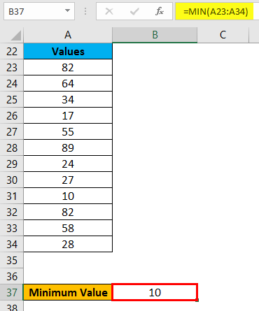
Now you can find out the range of the dataset after taking the difference between Maximum and Minimum value.
We can reduce the steps for calculating the range of a dataset by using the MAX and MIN functions together in one line.
For this, we again take an example to understand the process.
Range in Excel – Example #4
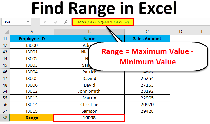
Let’s assume the below dataset of a company employee with their achieved sales target.
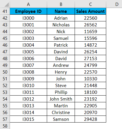
Now for identifying the span of sales amount in the above dataset, we will calculate the range. For this, we will follow the same procedure as we did in the above examples.
We will apply the MAX and MIN functions for calculating the Maximum and Minimum sales amount in the data.
For finding the range of sales amount, we will apply the below formula:
Range = Maximum Value – Minimum Value
Refer to the below screenshot:
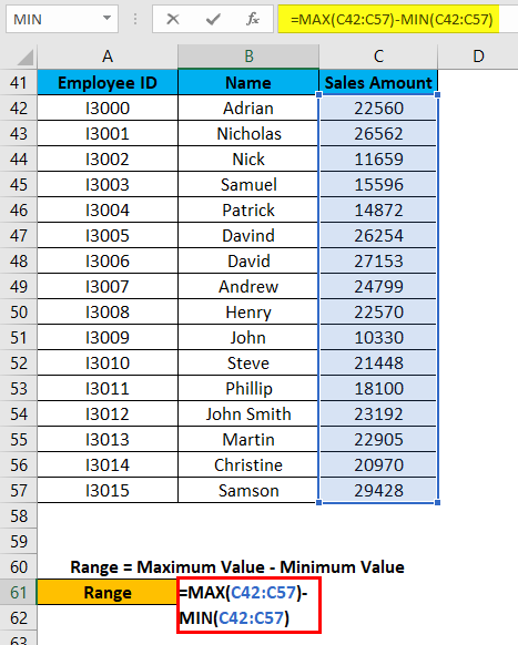
Press Enter key, and it will give you the range of the dataset. The result is shown below:
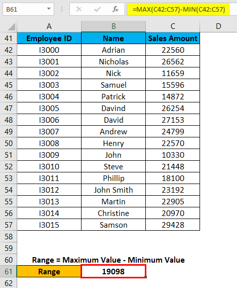
As we can see in the above screenshot, we applied the MAX and MIN formulas in one line, and by calculating their results difference, we found the range of the dataset.
Things to Remember
- If the values are available in the non-adjacent cells, you want to find out the range; you can pass the cell address individually, separated with a comma as an argument of the MAX and MIN functions.
- We can reduce the steps for calculating the range by applying MAX and MIN functions in one line. (Refer to Example 4 for your reference)
Recommended Articles
This has been a guide to Range in Excel. Here we discuss how to find Range in Excel along with excel examples and downloadable excel template. You may learn more about Excel from the following articles –
Источник
Excel Function for Range
Excel Function for Range (Table of Content)
Range Function in Excel
Range in Excel is the difference between the maximum limit and minimum limit of the available numbers in excel. For example, we have around 10 different number of randomly selected in a list in Excel. To calculate the Range for these numbers, we need to find the upper and lower values using the MAX and MIN function in the list of those cells. Once we get the maximum and minimum values out of those numbers, then subtract the Max value from the Min value. The returned number will be the range.
Excel functions, formula, charts, formatting creating excel dashboard & others
There are two kinds of ranges used extensively in excel, which are illustrated below:
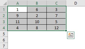
Symmetrical Range: A range which consists of all cells in adjacent positions to each other. Such a range usually shows up as a square or rectangle in a spreadsheet when highlighted. The range shown in the image would be (A1:C4)
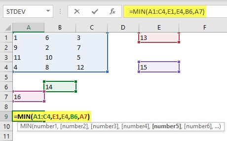
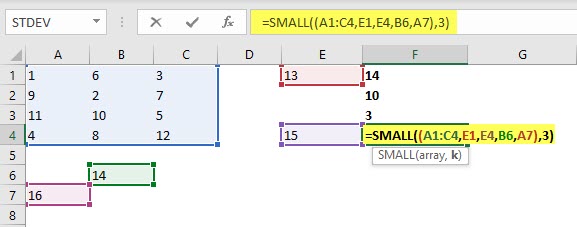
Irregular Range: A range consisting of cells that are not contiguous and may not have regular geometrical shapes when highlighted. The range highlighted in the image would be (A1:C4, E1,E4, B6,A7)

Examples of Range Function in Excel
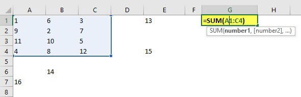
Now, a range in itself would not be useful as we have to derive insights from the range’s data. So formulae are used with cell ranges which add the operation we want to perform in the data from the range. For example, if we want to find the sum of the numbers in cells A1 till C4, .we would use =SUM(A1:C4)
Example #1 – Finding Maximum and Minimum
1) Finding the maximum and minimum values in a cell range: We use the following functions when we are looking for minimum and maximum values in a cell range. Please note that this would give us the mathematical result and not the maximum and minimum as defined by cell number.
- For Maximum: We would use the =MAX(Cell Range) function as illustrated below.
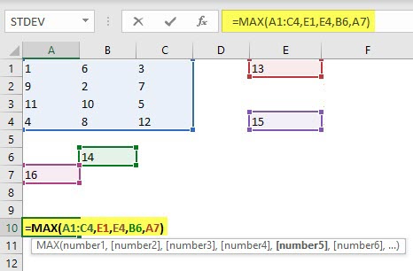
- For Minimum: We would use the =MIN(Cell Range) function as shown below.
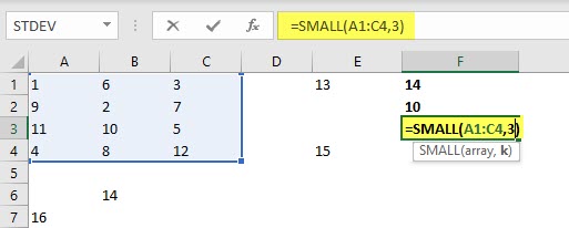
2) Suppose we are not interested just in the minimum and maximum in the highlighted range, but also in the top and bottom k numbers in the range. We can use the following functions to calculate those.
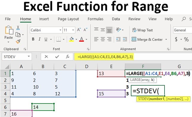
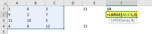
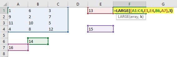
- For the top k number, say k=3, which means the third-largest number in the range, we would use the function =LARGE(Cell Array,k) for symmetrical ranges or =LARGE((Cell Range),k) for irregular ranges as shown below.
- A very similar function for finding the kth smallest number in a range would be to use =SMALL(Cell Array, k) for a symmetrical range or =SMALL((Cell Range),k) for an irregular range.
Example #2 – How to Define and Use Ranges in Excel?
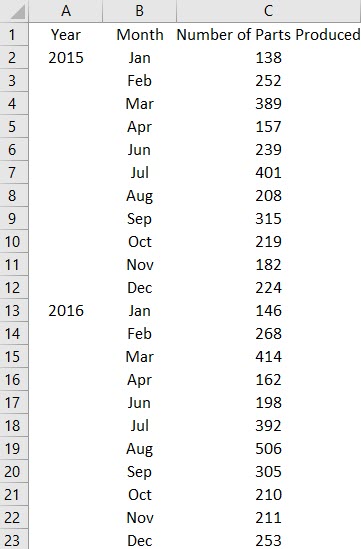
We will now look at how to define and use ranges in excel. First, we need to have data to work with. This can be anything in a spreadsheet ranging from letters to numbers or a combination of both. For the illustrations accompanying this discussion, I am using a sample from a production database which stores data on how many parts are produced in a year.
Let us say we want to know the range of production numbers that have been entered over the two years. We do this by subtracting the minimum from the maximum value. For this, we need not find each value individually but have to breakdown the calculation steps and write the formula as follows:
MAX(Cell Range)-MIN(Cell Range)
Please note that the cell range has to be the same in the arguments; otherwise, the formula would not return the correct result.
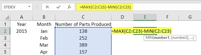
We find that the range of production is 368 parts. Now, if we want to find out the occurrence of a particular value in the range, or a range of values within the range, we use another function called COUNTIF. This function has the following syntax:
Let us suppose we want to find what was month in which we hit more than 300 parts. The formula would be =COUNTIF(C2:C23,”>300″)
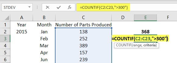
We find that for 7 months, the production was more than 300 parts. We can also find out if we had any month which was below a particular number, suppose 100. We would use a nested COUNTIF formula within an IF statement to get a Yes or No answer like this:
=IF(COUNTIF(range,” value”),” Yes”,” No”)
This would look like this:
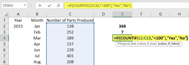
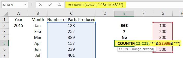
The result would be a No as none of the production numbers in the range is below 100. A variation of this can be used to find if we have any production number in a particular value. This would be as follows:
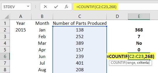
COUNTIF(range,”*”&value&”*”) or COUNTIF(range, value)
The first variation is useful if we want to match two different databases, and the second when we want to find out if a particular value occurs or not, and if it does, then how many times it reoccurs.
We can use the MATCH function instead of COUNTIF in case we want to find the number of values greater or less than a given value.
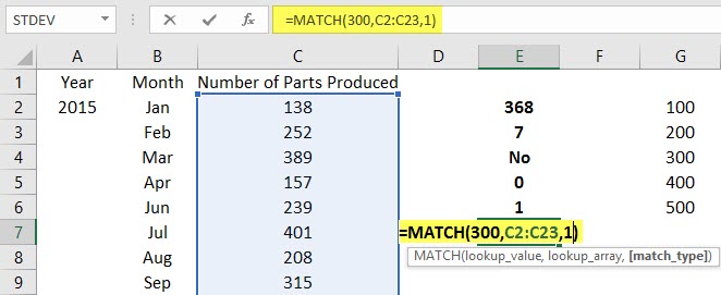
In the above example, we use the MATCH function to find the number of months that had less than 300 parts produced.
Things to Remember
- We should sort the data in ascending or descending order wherever feasible to simplify operations when using ranges.
- Quotation marks (“”) and asterisk(*) are used in formulae whenever we are looking for substrings or specific text ranges within a range.
- Irregular ranges are the most common ranges used in business. As such, whenever possible, we should use tables to classify the data before running any operations on them.
- It must be noted that ranges can be highlighted manually, and Excel displays the number of cells in it as a count at the bottom; however, we can find out the number of rows or columns in a range using the following functions:
Usually, these two functions are not required but are useful for large tables and multiple databases and for recording macros.
Conclusion
Knowledge of range in excel is an important pre-requisite to being able to manipulate data. The range is also used in recording macros and VBA coding, and hence an in-depth understanding of range is a must for anyone using excel.
Recommended Articles
This is a guide to Excel Function for Range. Here we have discussed Examples of Range Function in Excel along with steps and a downloadable excel template. You may also look at the following articles to learn more –
Источник
What is the Range Formula?
The range formula refers to the formula used to calculate the difference between the maximum and minimum values of the range. According to the formula, the minimum value is subtracted from the maximum value to determine the range.
Range = the maximum value – the minimum value
The given dataset provides statisticians and mathematicians with a better understanding of the data set and how varied it is. Moreover, it is the simplest approach to calculating variance in statistics.
Table of contents
- What is the Range Formula?
- Explanation
- Examples
- Uses of Range Formula
- Recommended Articles
Explanation
It is quite simple and easy to use as the formula states its maximum value less the minimum value of the given sample. Therefore, the range is the variance between the maximum and minimum values. However, even though that is simple to use and understand, it requires interpretation properly.
For example, if there is an outlier in the data, the range will be influenced by the same, leading to misrepresentation. Take a practical example for data 2, 4, 7, 7, and 100. Then, the range would be 100 – 2, which is 98, but as one can see that the data range lies below 10, considering and interpreting that data is within 98 will lead to misrepresentation. Hence, one should conduct the interpretation of range with due consideration.
Examples
You can download this Range Formula Excel Template here – Range Formula Excel Template
Example #1
Consider following given dataset 2,2,4,4, 4, 6,7,7,8, 8, 8, 9 ,9, 9, 9, 9. You are required to calculate the Range for this sample.
Solution:
- Maximum value = 9
- Minimum value = 2
Range = 9 – 2
Range = 7
Example #2
Mr. Stark is a scientist who has worked for 10 years with a Dream Moon company. Mr. Arora, his supervisor, is experimenting with human health and has collected a few sample data of male height, which are 162, 158, 189, 144, 151, 150, 151, 178, 155, and 160. He is perplexed now and wants to know how much data is varied. Mr. Stark, an experienced statistician, has been approached by his supervisor Mr. Arora to remove his confusion about the formula variation. Mr. Arora is required to provide an answer to his supervisor. You are required to calculate how much the data varied.
Solution:
Range = maximum value – minimum value
- Maximum value = 189
- Minimum value = 144
Range = 189 – 144
Range = 45
The data or the sample collected has a variation of 45.
Example #3
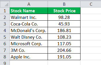
Mr. Buffet, a well-known and esteemed investor worldwide, is now considering US market stock and is analyzing a few of them in where he wants to invest. The list includes major blue-chip companiesBlue chip stocks are issued by companies possessing large market capitalization. Blue chip companies are market leaders. They provide good returns on stocks, offer dividends, and are considered safe investments.read more in the US. Below are the given shortlisted stocks or securities along with their latest stock market price, denoted in US$, where he is considering investing.
You are required to calculate Range and come up with the variation the list has.
Solution:
Below is given data for calculation of the range.
Using the above information, the calculation of Max Value in excelThe MAX Formula in Excel is used to calculate the maximum value from a set of data/array. It counts numbers but ignores empty cells, text, the logical values TRUE and FALSE, and text values.read more will be as follows,
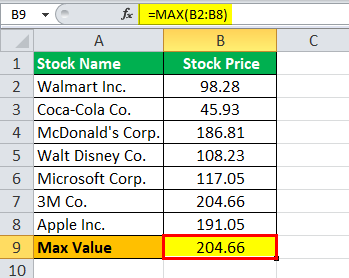
Max Value = 204.66
Calculation of Min Value in excelIn Excel, the MIN function is categorized as a statistical function. It finds and returns the minimum value from a given set of data/array.read more as follows,
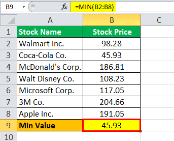
Min Value = 45.93
Therefore, the calculation of range is as follows,
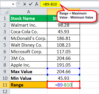
Range = 204.66 – 45.93
The range will be –
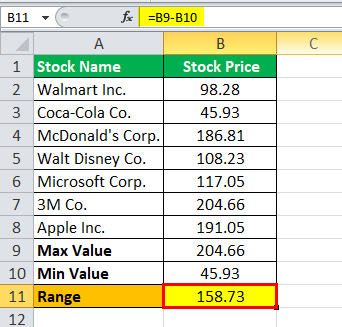
Range = 158.73
Uses of Range Formula
The range is a very easy and basic understanding of how the numbers in the given data set or sample spread out because, as stated earlier, it is relatively easy to calculate since a very basic arithmetic operation is only required to subtract the minimum from the maximum value. Still, the range has few more applications for a given data set or a given sample in statistics. For example, the range is also useful in estimating another measure of spread, called variance or the standard deviation.
The range, as mentioned earlier, can only inform about the basic details, i.e., where the spread of a given sample or set of data will lie. Giving the difference or, say, the variance between the highest and the lowest values of a given sample or given dataset gives information or a rough idea about the significant extreme observations of how widely spread out those are. Still, again it gives no hint or any information as to the other data points where they would lie, which is the main weakness of using the range equation.
The range, as discussed above, is useful for depicting the spread within a given sample or dataset. Further, one may use it to compare the resultant spread between the same given sample or datasets.
Recommended Articles
This article has been a guide to Range Formula. Here, we discuss calculating the range using its formula, Excel examples, and a downloadable Excel template. You can learn more about financing from the following articles: –
- Standard Deviation FormulaStandard deviation (SD) is a popular statistical tool represented by the Greek letter ‘σ’ to measure the variation or dispersion of a set of data values relative to its mean (average), thus interpreting the data’s reliability.read more
- FormulaA sampling distribution is the probability-based distribution of detailed statistics. It helps calculate means, range, standard deviation, and variance for the undertaken sample. For a sample size of more than 30, the formula is: µ͞x =µ and σ͞x =σ / √n
read more of Sampling DistributionA sampling distribution is the probability-based distribution of detailed statistics. It helps calculate means, range, standard deviation, and variance for the undertaken sample. For a sample size of more than 30, the formula is: µ͞x =µ and σ͞x =σ / √n
read more - Midrange FormulaMidrange formula is used in order to calculate the middle value of the two number given and according to the formula the given two number are added and the resultant is divided by the 2 in order to get the midpoint value of the two.read more
- Amortized LoanThe amortized loan formula is used to calculate the annual or monthly payments a borrower must make to the lender for the loan they have taken out. Annual interest payments plus the annual portion of the long-term debt make up the yearly payment.read more