
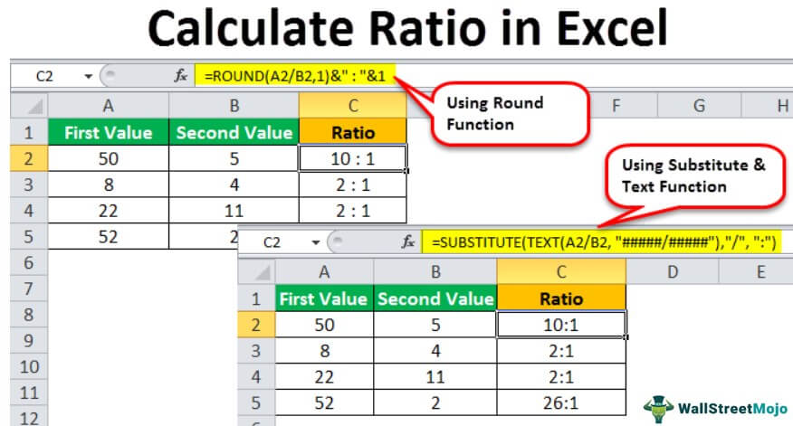
Calculate Ratio in Excel Formula
The ratio usually compares the values. It helps us to tell how much one value is smaller or bigger than the other. In mathematics, a ratio is a relationship between two values showing how many times the first value contains the additional value.
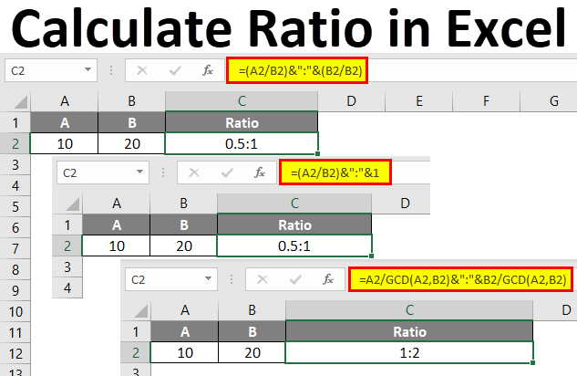
For example, suppose in a dataset, we have the value 5 in cell A2 and 30 in cell B2, and we need to determine the ratio. In this scenario, we can use the RATIO formula in Excel. In this example, we can use the following formula in cell C2:
=(A2/B2)&”:”&(B2/B2)
=1:6.
It helps to define the comparisons between two different values or things.
In Excel, there is no specific function to calculate the ratio. Instead, there are four functions to calculate the ratio in the Excel formula, which we can use per the requirements.
Following are the functions to calculate the ratio in the excel formula:
- Simple Divide Method.
- GCD Function.
- SUBSTITUTE and TEXT Function.
- Using ROUND Function.
Table of contents
- Calculate Ratio in Excel Formula
- How to Calculate Ratio in Excel?
- #1 – Simple Divide Function
- Example of Simple Divide Function
- #2 – GCD Function
- Example of GCD Function
- #3 – SUBSTITUTE and TEXT Function
- Example of SUBSTITUTE and Text Function
- #4 – ROUND Function
- Example of Round Function
- Things to Remember while Calculating Ratio in Excel Formula
- Recommended Articles
How to Calculate Ratio in Excel?
Let us learn how to calculate the ratio in the Excel formula with the help of a few examples of each function.
You can download this Ratio Calculation Excel Template here – Ratio Calculation Excel Template
#1 – Simple Divide Function
The formula for the Simple Divide Method in ExcelDivide in Excel is used for division applications, where (/) is the symbol and we can write an expression =a/b, where a and b represent two numbers or values to be divided.read more:
= value1/ value2 &”:“&“1”
Example of Simple Divide Function
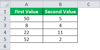
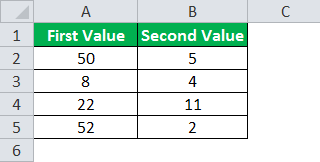
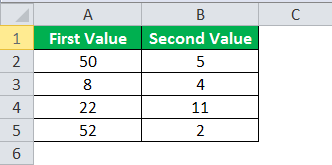
We have data where we have two values. We will have to calculate the ratio of the two numbers.
Steps to calculate the ratio in Excel formula with the help of the simple divide function are shown below:
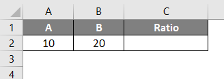
- Data with two values, as shown below:
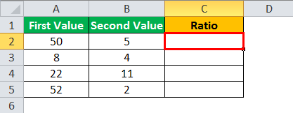
- Now, select the cell in which you want the ratio of the given values, as shown below.
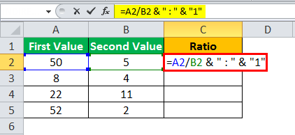
- Now, use simple divide function to calculate the ratio as =first value/second value&” : “ & “1”.
- Press the “Enter” key to see the result after using the simple divide function.
- Now, drag the function to the below cells to calculate the ratio of complete data and find the result as shown below.
#2 – GCD Function
A formula for GCD Function:
= value1 / GCD (value1, value2) &”:“& value2 / GCD (value1, value2)
Example of GCD Function
We have data where we have two values. We will have to calculate the ratio of two numbers in Excel.
Steps to calculate the ratio in Excel formula with the help of the GCD function are shown below:
- Data with two values, as shown below:
- First, calculate the GCD to make it less complicated than GCD (first value, second value).

- Now, use the GCD function method to calculate the ratio as =first value/ GCD (first value, second value) & ” : “ & second value/ GCD (first value, second value).
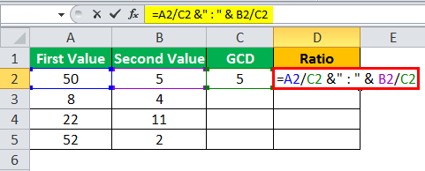
- Press the “Enter” key to see the result after using the GCD function.
- Now, drag both the functions to the below cells to calculate the ratio of complete data and find the result as shown below.
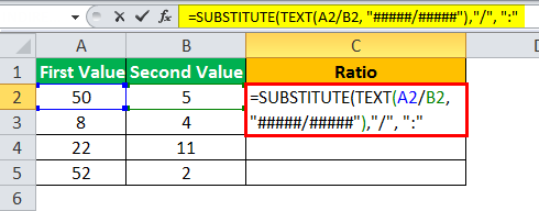
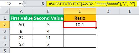
#3 – SUBSTITUTE and TEXT Function
A formula using the SUBSTITUTE Function in excelSubstitute function in excel is a very useful function which is used to replace or substitute a given text with another text in a given cell, this function is widely used when we send massive emails or messages in a bulk, instead of creating separate text for every user we use substitute function to replace the information.read more and Text Function in excelTEXT function in excel is a string function used to change a given input to the text provided in a specified number format. It is used when we large data sets from multiple users and the formats are different.read more.
= SUBSTITUTE (TEXT (value1/value2, “#####/#####”),”/”, “:”)
Example of SUBSTITUTE and Text Function
We have data where we have two values. We will have to calculate the ratio of the two numbers.
Steps to calculate the ratio with the help of the SUBSTITUTE and TEXT functions are shown below:
- Data with two values, as shown below:
- Now, select the cell in which you want the ratio of the given values, as shown below.
- Now, use the SUBSTITUTE and TEXT function to calculate the ratio as =SUBSTITUTE(TEXT(first value/second value, “#####/#####”),”/”, “:”).
- Press the “Enter” key to see the result after using the SUBSTITUTE and TEXT functions.
- Now, drag the function to the below cells to calculate the ratio of complete data and find the result as shown below.
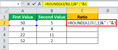
#4 – ROUND Function
A formula for Round Function.
= ROUND (value1/value2, 1) &“:”& 1
Example of Round Function
We have data where we have two values. We will have to calculate the ratio of the two numbers.
Steps to calculate the ratio of two numbers with the help of the ROUND function are shown below:
- Data with two values, as shown below:
- Now, select the cell in which you want the ratio of the given values, as shown below.
- Now, use the ROUND function to calculate the ratio as =ROUND( first value/second value,1)&“:”&1
- Press the “Enter” key to see the result after using the ROUND function.
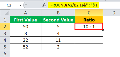
- Now, drag the function to the below cells to calculate the ratio of complete data and find the result as shown below.
Things to Remember while Calculating Ratio in Excel Formula
- There should be numeric values for which you want to calculate the ratio in Excel.
- Both the values should be positive, and the second should not be zero.
- There is no specific function to calculate the ratio; as per the requirement, we can use the functions.
Recommended Articles
This article is a guide to Calculate Ratio in Excel formula. Here, we discuss calculating ratios in Excel using 1) Simple Divide function 2) GCD function 3) SUBSTITUTE and TEXT functions, and 4) ROUND function with examples and downloadable Excel templates. You may also look at these useful functions in Excel: –
- Calculation of Percent Error FormulaPercentage error formula is calculated as the difference between the estimated number and the actual number in comparison to the actual number and is expressed as a percentage, to put it in other words, it is simply the difference between what is the real number and the assumed number in a percentage format.read more
- Multiply in ExcelMultiplication in excel is performed by entering the comparison operator “equal to” (=), followed by the first number, the “asterisk” (*), and the second number.read more
- Subtraction Formula in ExcelThe subtraction formula in excel facilitates the subtraction of numbers, cells, percentages, dates, matrices, times, and so on. It begins with the comparison operator “equal to” (=) followed by the first number, the minus sign, and the second number. For example, to subtract 2 and 5 from 15, apply the formula “=15-2-5.” It returns 8.read more
- “Not Equal to” in Excel
A ratio is one of the common methods to compare two values with each other. And it can help you to compare variations between those two values.
Even in our daily life, we use the word RATIO to define the comparison between two different things. When it comes to Excel, we don’t have any specific single function which can help us to calculate a ratio.
But you can calculate it using some custom formulas. So today, in this post, I’d like to show you how to calculate ratios using 4 different ways.
Let’s get started and make sure to download this sample file from here to follow along.
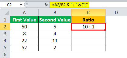
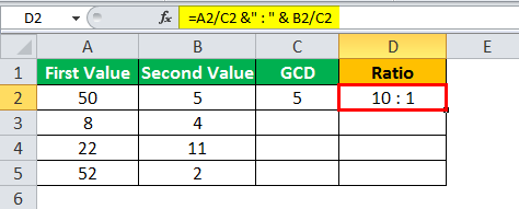
1. Calculate the Ratio by using the Simple Divide Method
We can use this method when the larger value is divisible by the smaller value. In the below example, we have values 10 and 2, where 10 is divisible by 2.

So you can use this method here. Insert the below formula into the cell and hit enter.
=A2/B2&":"&"1"
here’s how this formula works…
In this formula, we have divided 10 by 2 which gives you 5 in return. So now we have 5 instead of 10 by dividing by 2. And on the other side, we have used 1 instead of 2.

- PROs: #1. Simple to apply. #2. Easy to understand.
- CONs: #1. Limited use. #2. Not applicable if the larger value is not divisible by the smaller value.
2. GCD Function to Calculate Ratio in Excel
As I said, there is no single function in excel to calculate the ratio for you. But, the GCD function is close enough.
It can help you to get a common denomination for both of the values and then by using a little concatenation, you can calculate the ratio.

And to calculate the ratio insert the below formula into the cell and hit enter.
=A2/GCD(A2,B2)&":"&B2/GCD(A2,B2)
here’s how this formula works…
Maybe it looks complex to you but it’s simple in reality. Let me explain this in two parts.

As I said, GCD can give you a common denominator for both of the values. So here you have to use GCD in both of the parts of the formula to get a common denominator.
After that, you have to divide both of the values with that common denominator. And, in the end, a little concatenation to join both of the values using a colon.
- PROs: #1. It’s a dynamic formula, it doesn’t matter even if you change the values. #2 Easy to apply.
- CONs: #1. GCD function only works with integers and if you have decimals in your values, it will not work.
3. SUBSTITUTE and TEXT for Ratio Calculation
A combination of two awesome functions. Yes, you can use the SUBSTITUTE and TEXT functions to calculate the ratio. This method works like a charm just like the GCD function. Here we have the below values to calculate the ratio.

In a cell, insert the below formula and hit enter.
=SUBSTITUTE(TEXT(A2/B2,"#####/#####"),"/",":")
here’s how this formula works…
This formula also works in two different work parts TEXT and SUBSTITUTE.

First, you have to use the text function to divide both of the numbers, and after that format the returning value in a fractional format.
Second, by dividing both of the values you have got 10 and when you convert this value into a fractional part you will get 10/1.
Third, replace the forward slash with a colon. And, we have a substitute function for that.
- PROs: #1. A dynamic formula doesn’t matter even if you change the values. #2. Simple to use and understand.
- CONs: If you have simple values to calculate a ratio, it’s not good to use this method.
4. Calculate the Ratio with Round Function
Using the round function to calculate a ratio is also a useful method. This is especially useful when you want to calculate ratios with decimals for accurate comparison.
Here we have values in which the higher value is not divisible by the smaller value. So, in this situation instead of using them as they are you can divide them and show the final ratio with decimals.

Just insert the below formula into the cell and hit enter.
=ROUND(A2/B2,1)&":"&1
And, here you have a ratio with decimals.
here’s how this formula works…
You can split this formula into two different parts to understand it. First of all, you have to use the round function to divide the larger value by the small value and get the result with one decimal. Second, you have to use a colon and “1” at the end.
- PROs: #1. Useful when you want to get results with decimals. #2. The final value will be more accurate.
- CONs: #1. Not applicable in all situations.
Sample File
sample file
Conclusion
As I said, a ratio is a useful method to compare two values with each other. And now, you have different methods to calculate it in your favorite application, yes, in Excel.
All the methods which we have used above can help you to calculate ratios in different situations with different types of values.
I hope this will help you in your work. Now, tell me one thing. Do you have any other method to calculate the ratio? Please share with me in the comment section, I would love to hear from you.
And, please don’t forget to share this tip with your friends. I’m sure they will appreciate it.
Introduction to Ratio in Excel
A ratio is a way to compare two data sets that allow us to get which data is greater or lesser. It also gives the portion between 2 parameters or numbers. By this, we can compare the two data sets.
Calculate Excel Ratio (Table of Contents)
- Introduction to Ratio in Excel
- How to Calculate Ratio in Excel?
- Pros of Calculating Ratio in Excel
How to Calculate Ratio in Excel?
Calculate the Ratio in excel is very simple and easy. Let’s understand how to calculate ratios in excel with some examples.
You can download this Ratio Excel Template here – Ratio Excel Template
Calculate Ratio in Excel – Example #1
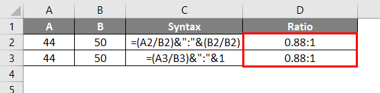
The calculating Ratio in excel is simple, but we need to understand the logic of doing this. Here we have 2 parameters, A and B. A has a value of 10, and B has a value as 20, as shown below.
And for this, we will use a colon (“:”) as a separator. So for this, go to the cell where we need to see the output. And type the “=” sign (Equal) to go to the edit mode of that cell. In the first syntax, divide cell A2 with B2; in the second syntax, divide cell B2 with B2. Doing this will create the short comparative values to have a short ratio value, as shown below.
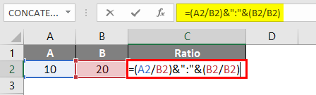
Note: & is used for concatenation of both the syntaxes and the colon (:) is the ratio symbol fixed between concatenation formulas.
Once done with syntax preparation, press Enter to see the result as shown below.
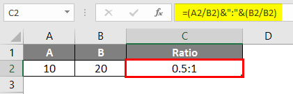
As we can see above, the calculated value of the Ratio is coming 0.5:1. This value can further be modified to look better by multiplying the obtained Ratio with 2 to have a completely exact value, not in fraction or else. We can keep it in its original form.
Calculate Ratio in Excel – Example #2
There is another method of calculating the Ratio in excel. We will consider the same data which we have considered in example-1. If we see the syntax we have used in example-1, we have divided cell B2 with B2.
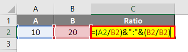
By dividing cell B2 with B2 or any cell with the same value, that cell gives the output as 1. The obtained Ratio in example-1 is 0.5:1, where value 1 is a division on 20/20 if we mathematically split the syntax. And 0.5 is the division of 10/20. This means if we keep 1 by default in the second syntax (Or 2nd half of the syntax), we will eventually get value 1 as a comparative of the First syntax (Or 1st half of the syntax).
Now, let’s apply this logic to the same data and see what result we get.
For this, go to the cell where we need to see the output and type the “=” sign. Now in the first half of the syntax, divide the cell A2 with B2, and in the second half of the syntax, put only “1,” as shown below.
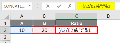
As we can see in the above screenshot, we have kept “1” in the second half of the syntax, creating the same value as example-1. Now press Enter to see the result.
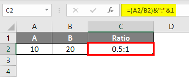
As we can see in the below screenshot, the obtained result is the same result we got in example-1.
Now verify both the applied formulas in example-1 and example-2; we will test them with a different value in both the syntaxes. For testing, we kept 44 in cells A2 and A3 and 50 in cells B2 and B3. And in both ways of calculating the Ratio, we are getting the same value in excel, as shown below.
Calculate Ratio in Excel – Example #3
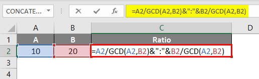
There is another method for calculating the Ratio in excel. This method is a little complex with short syntax. In excel, there is a format of finding the Greatest Common Divisor, which means when we select two values and then compare them with the third one, it automatically considers the greatest value from which that comparative ratio value will get divided. This we have done manually in example-1 and example-2. For this also, we will consider the same data which we have seen in the above examples.

Now go to the cell where we need to see the result and type the “=” sign. Now select cell A2 and divide it with GCD. And in GCD, select both cells A2 and B2. The same procedure follows for the second half of the syntax. Select cell B2 and divide with GCD. And in GCD, select both cells A2 and B2 separated by a comma (,) as shown below.
Once we do that, press Enter to see the result, as shown below.
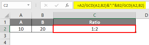
As we can see above, the calculated Ratio is coming as 1:2. The Ratio calculated in example-1 and example-2 is practically half of the Ratio coming in example-3 but has the same significance in reality. Both values carry the same features.
Not let’s understand the GCD function. GCD or Greatest Common Divisor in excel automatically finds the most outstanding value to divide it with the value present in the numerator. She is eventually giving the same result in methods used in example-1 and example-2.
Pros
- The methods shown in all the examples are easy to use.
- It is easy to understand the syntax and value entered.
- We can modify the syntax as per our requirements.
- If there are more than three values, it needs to be compared, and for that, we can use the same formula.
- A good thing about calculating the Ratio with GCD in excel is that it gives a result that looks good in terms of numbers, characters, and numbers.
Things to Remember
- Make sure the concatenation is done correctly to avoid errors.
- We can use the proper CONCATENATION formula instead of using & as a separator.
- A value obtained in example-1 and two and example-3 seems different, but technically there is no difference in all the ratio values.
Recommended Articles
This has been a guide to Calculate Ratio in Excel. Here we discuss how to calculate Ratio in Excel along with practical examples and a downloadable excel template. You can also go through our other suggested articles –
- FV Function in Excel
- CONCATENATE in Excel
- Simple Formula in Excel
- Divide Cells in Excel
This tutorial will show you how to compare two numbers and calculate their ratio, such as 5:7 or 8:3.
In this Article
- Calculate a Ratio – The GCD Method
- Using the GCD Function
- Calculate a Ratio – The Text & Substitution Method
Calculate a Ratio – The GCD Method
The GCD Function is used to calculate the greatest common denominator between two or more values. We can use GCD to then create our ratios.
To use the GCD Function, you may need to enable the Data Analysis Toolpak. To check if you will need to enable the Data Analysis Toolpak, type =gcd( into an Excel cell. If you see the GCD function inputs appear:
you are ready to begin. Otherwise follow the steps below:
For Mac
• Click on Tools. (Located at the very top where you have File and Edit.)
• Click on “Excel Add-ins.
• A small pop tab should appear. Be sure that Analysis ToolPak is selected.
• Select OK.
• The ToolPak should now be available in the Data tab with the title “Data Analysis.” If you do not see it, you may need to reload your page and check again.
For PC
• Click the File button
• Find and select Options. (It is located near the bottom.)
• On the left side click Add-Ins
• Under Inactive Applications find and select Analysis ToolPak
• Click Go
• A new window titled “Add-Ins” should appear. Select Analysis ToolPak.
• Click OK
• The ToolPak should now be available in the Data tab with the title “Data Analysis.”
Using the GCD Function
The GCD Function is extremely easy to use. Simply type =GCD( followed by the numbers that you wish to find the greatest common divisor of (separated by commas).
=GCD(Number 1, Number 2)
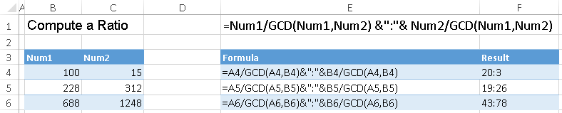
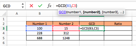
For example, our first row would be calculated as: =GCD(B3,C3) with the answer being 5.
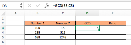
Once you understand how GCD works you can use the function to find your ratios by dividing each of the two numbers by their GCD and separating the answers with a colon “:”.Keep in mind that the answer will be a text value.
The formula for the ratio is:
= Num1/GCD(Num1, Num2) & “:” & Num2/GCD(Num1, Num2)
This complicated formula is basically saying,
= (Number of times Number 1 contains GCD) & “:” & (Number of times Number 2 contains GCD)
In our example the formula would be written as:
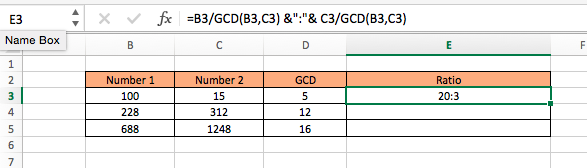
=B3/GCD(B3,C3) & ”:” & C3/GCD(B3,C3)
Which results in:
=100/5 & “:” & 15/5
= 20 & “:” & 3
= 20:3
Calculate a Ratio – The Text & Substitution Method
Another method to calculate ratios is the Text & Substitution Method. This method does not require the Analysis ToolPak to be installed.
The Text Function allows you to display an answer as a text value. In our case it will divide Number 1 by Number 2, but instead of producing a decimal value the answer will be displayed as a fraction, such as 5/4 or 9/2.
The formula for the fraction is:
=TEXT(Number 1/Number 2, “#/######”)
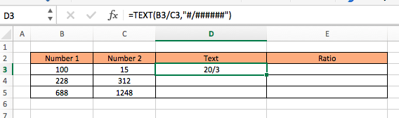
The Text Function tells Excel to display the answer in the form “num1/num2” The extra ##### in the Text formula tells Excel to display the largest fraction. If you only specify #/# you may receive a rounded answer because Excel will display a fraction with only one digit for the numerator and denominator.
To display the fraction in the desired ratio format you will have to substitute the slash with a colon. This will involve using the Substitution Function.
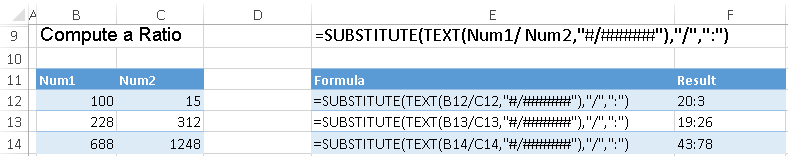
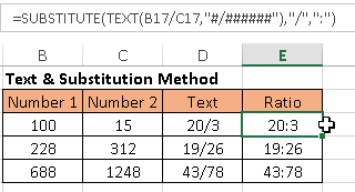
=SUBSTITUTE(TEXT(Num1/Num2, “#/######”),”/”,”:”)
In our example this would be written as:
=SUBSTITUTE(TEXT(B3/C3, “#/######”),”/”,”:”)
This results in:
=SUBSTITUTE(TEXT(100/15, “#/######”),”/”,”:”)
= 20:3
A ratio shows the quantitative relation between two positive numeric values, indicating how many times one number contains the other. More commonly, you may be accustomed to seeing ratios expressed as a fraction e.g. 1:3 holding the equivalence of 1/3.
Whether as a fraction, decimal, or with the ratio symbol, ratios have wide use in mathematics and even in the business world. The concept of ratios is paramount for analysis and you might be familiar with financial ratios (liquidity, profitability, efficiency ratios, etc.) in business, win/loss ratio in sports and games, or a simple ratio for quantitative measures in baking, measurement, etc.
Excel doesn’t have any function or feature as yet for calculating a ratio itself. Nonetheless, we can get our way around with some Excel tricks by using certain functions as part of simple formulas. We’ll demonstrate 4 methods of calculating ratios in Excel; namely, they are the division method and the GCD, SUBSTITUTE & TEXT, and the ROUND functions. Ready to dive in?
Let’s get calculating!
 1")
Number 1 as Denomination
Taking a small example, if you were to calculate the ratio of the numbers 60 and 120, it would be 1:2. This is the most typical form of ratios, with the terms of the ratios in the simplest form of divisors. This ratio can also be written as 0.5:1 in which case, the purpose of the ratio is to have the number 1 as the denomination.
This method may be required to keep the base stable and find the relative quantity of the other number against 1. We have a couple of methods under this form of ratio. Let’s find out what they are.
Using Division Method
Beginning with the basic concept of ratios, our first method uses division to arrive at a ratio of one value against the other. The purpose of this method is not only to divide the values but also to determine the ratio against the number 1 as explained above.
We require the consequent to remain 1 and will aim to find the antecedent by dividing one value from the other. If this is confusing you, let us show you an example; it’s actually much easier than it sounds. Even if you were a math and stats backbencher, you’ll get hold of this in no time. See the formula below:
=C3/D3&":1"
Espresso guide below. Let’s admit it, if you’ve never come across this before, you’re thrilled right now (or enlightened, to say the least). The guide shows the measurements of brewed coffee (mostly an espresso shot) and milk in various coffee beverages. Since it would be incredibly helpful to have their ratios, we’ve wasted no time in calculating them.
Using the aforementioned formula, the values in column C have been divided by the values in column D. Dividing C3 by D3 (60/30) gives us 2. Now, to place this value against the number 1, we have used the & operator to add two text elements. The first is the classic ratio sign, the colon “:”. Along with that, we’ve added the number 1. The results of using this formula to calculate ratios in our example have turned out like this:
 2")
That was neat but matters aren’t always going to be as straightforward as this. You won’t always be working with numbers that produce clear-cut integers and decimals. If that’s the case for you, you can still use this formula with the ROUND function. In fact, we can show you how it’s done.
Using ROUND Function
Calculating ratios is easy with the help of the ROUND function. How does the ROUND function help? The ROUND function rounds a number off to the mentioned number of digits. The number of digits mentioned as a positive integer will round the number off to the integer number of decimal places.
For our second example, the ROUND function will be well handy to get, let’s say a maximum of 2 decimal places. Why must you use the ROUND function and not adjust the result by decreasing the decimals or applying a number format? That is because only part of the result will be a decimal; the rest will be affixed text and therefore, the result as a whole can’t be given a number treatment. Hence, we need the ROUND function to take care of the decimal beforehand. See how it happens:
=ROUND(E3/F3,2)&":1"
The formula itself is quite like the previous one, only with the ROUND function added. And why is it added? Cast a look at the example below. 10 teams have played a certain number of matches (listed in column C) and the matches won and lost by them have been jotted down in columns E and F. Looking at the numbers on their own doesn’t give us an instant understanding of the teams’ performances.
Calculating the win to loss ratio would be ideal and is achievable with the simple division method. But if the results carry several decimal places, the data would be hard to read. Consequently, the ROUND function has been added to the formula where it divides E3 by F3 and sets the decimal places to 2 digits. This takes the original answer of the division from 1.722222222 down to 2 decimal places as 1.72.
Next, the & operator joins the text string “:1” to the result of the ROUND function and the outcome is 1.72:1. This implies that for every loss, Team C has at least more than one victory. The rest of the ratios calculated using the ROUND function for the teams follow as:
 3")
Note: You could even set the decimal places in the ROUND function to one digit but for our scenario, it’s best to have 2 decimal places. If we look at Team B and D’s ratios, had there been only 1 decimal place to display, 1.24 would be rounded down to 1.2, and 1.16 would be rounded up to 1.2 as well. This would have made both teams’ win-loss ratios look identical. For a better assessment of the performance of the teams, 2 decimal places would be apt. You can choose to set more or lesser decimal places as per your data.
Terms of Ratio in Simplest Form
A ratio is said to be is the simplest form when the numbers are expressed as natural numbers with no common factor between them.
Using GCD Function
The ratios we just saw were very filtered down because the ratio had to be denominated by the number 1. As per your requirement, you may need the terms of the ratio to be in their simplest form of divisors instead of 1 as the denomination. For the latter type, you can calculate ratios with the GCD function.
The GCD function returns the greatest common divisor. The greatest common divisor of both numbers will be used to find a common denominator in the numbers. The common denominators will make up the terms of the ratio. The formula below will show you how to use the GCD function to calculate ratios:
=E3/GCD(E3,F3)&":"&F3/GCD(E3,F3)
We need two results from this formula that will be conjoined with a colon to arrive at the ratio. But if we process the GCD part first, the rest of the formula becomes quite simple to understand. The GCD of the numbers E3 and F3 has been calculated by the GCD function as 1. Since there is no common divisor, the number 1 has been returned. Now E3 is divided by 1 and F3 is also divided by 1, resulting in 31 and 18 respectively.
These results have been pieced together by the & operator but for the ratio effect, of course we require the colon. The output of the formula is 31:18. Here you can see how the GCD function has helped us to calculate the win/loss ratios for our example case:
 4")
Using SUBSTITUTE & TEXT Functions
This is another easy way to calculate ratios that will produce results identical to the GCD function. And that is by using the SUBSTITUTE and TEXT functions. The SUBSTITUTE function replaces the specified text with new text. The TEXT function converts a value into text using the provided number format.
How is that going to work for us? The first step is to convert the two individual numbers in E3 and F3 into a recognized number format, in this case, into a fraction. Then the SUBSTITUTE function can replace the forward-slash (/) in the fraction with a colon (:). That will effectively change the fraction into a ratio. This is the formula you can use to calculate a ratio using the SUBSTITUTE and TEXT functions:
=SUBSTITUTE(TEXT(E3/F3,"#/######"),"/",":")
The TEXT function starts off by taking the numbers 31 and 18 and converting them into a fraction as per the given number format «#/######”. We have the fraction 31/18 now. The SUBSTITUTE function replaces the forward-slash in 31/18 with a colon to form the ratio. The final result is 31:18. The other ratios calculated using this formula with the SUBSTITUTE and TEXT functions are shown as follows:
 5")
Are you good to calculate ratios in Excel now? We thought so too. With the right Excel tricks in hand, you should be tossing over ratios in no time.
If you find yourself a little lost on what to do next time you’re computing ratios, you can remember that ratios can be expressed as fractions which can be converted to ratios. Good trick, is it not? Want to master other Excel tasks? There’s a profusion to explore and we’ll be back with +1 to that profusion to clear some Excel confusion.