
Excel for Microsoft 365 for Mac Excel 2021 for Mac Excel 2019 for Mac Excel 2016 for Mac Excel for Mac 2011 More…Less
If you receive information in multiple sheets or workbooks that you want to summarize, the Consolidate command can help you pull data together onto one sheet. For example, if you have a sheet of expense figures from each of your regional offices, you might use a consolidation to roll up these figures into a corporate expense sheet. That sheet might contain sales totals and averages, current inventory levels, and highest selling products for the whole enterprise.
To decide which type of consolidation to use, look at the sheets you are combining. If the sheets have data in inconsistent positions, even if their row and column labels are not identical, consolidate by position. If the sheets use the same row and column labels for their categories, even if the data is not in consistent positions, consolidate by category.
Combine by position
For consolidation by position to work, the range of data on each source sheet must be in list format, without blank rows or blank columns in the list.
-
Open each source sheet and make sure that your data is in the same position on each sheet.
-
In your destination sheet, click the upper-left cell of the area where you want the consolidated data to appear.
Note: Make sure that you leave enough cells to the right and underneath for your consolidated data.
-
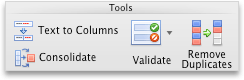
On the Data tab, in the Data Tools group, click Consolidate.

-
In the Function box, click the function that you want Excel to use to consolidate the data.
-
In each source sheet, select your data.
The file path is entered in All references.
-
When you have added the data from each source sheet and workbook, click OK.
Combine by category
For consolidation by category to work, the range of data on each source sheet must be in list format, without blank rows or blank columns in the list. Also the categories must be consistently labeled. For example, if one column is labeled Avg. and another is labeled Average, the Consolidate command will not sum the two columns together.
-
Open each source sheet.
-
In your destination sheet, click the upper-left cell of the area where you want the consolidated data to appear.
Note: Make sure that you leave enough cells to the right and underneath for your consolidated data.
-
On the Data tab, in the Data Tools group, click Consolidate.
-
In the Function box, click the function that you want Excel to use to consolidate the data.
-
To indicate where the labels are located in the source ranges, select the check boxes under Use labels in: either the Top row, the Left column, or both.
-
In each source sheet, select your data. Make sure to include either the top row or left column information that you previously selected.
The file path is entered in All references.
-
When you have added the data from each source sheet and workbook, click OK.
Note: Any labels that don’t match labels in the other source areas cause separate rows or columns in the consolidation.
Combine by position
For consolidation by position to work, the range of data on each source sheet must be in list format, without blank rows or blank columns in the list.
-
Open each source sheet and make sure that your data is in the same position on each sheet.
-
In your destination sheet, click the upper-left cell of the area where you want the consolidated data to appear.
Note: Make sure that you leave enough cells to the right and underneath for your consolidated data.
-
On the Data tab, under Tools, click Consolidate.
-
In the Function box, click the function that you want Excel to use to consolidate the data.
-
In each source sheet, select your data, and then click Add.
The file path is entered in All references.
-
When you have added the data from each source sheet and workbook, click OK.
Combine by category
For consolidation by category to work, the range of data on each source sheet must be in list format, without blank rows or blank columns in the list. Also the categories must be consistently labeled. For example, if one column is labeled Avg. and another is labeled Average, the Consolidate command will not sum the two columns together.
-
Open each source sheet.
-
In your destination sheet, click the upper-left cell of the area where you want the consolidated data to appear.
Note: Make sure that you leave enough cells to the right and underneath for your consolidated data.
-
On the Data tab, under Tools, click Consolidate.
-
In the Function box, click the function that you want Excel to use to consolidate the data.
-
To indicate where the labels are located in the source ranges, select the check boxes under Use labels in: either the Top row, the Left column, or both.
-
In each source sheet, select your data. Make sure to include either the top row or left column information that you previously selected, and then click Add.
The file path is entered in All references.
-
When you have added the data from each source sheet and workbook, click OK.
Note: Any labels that don’t match labels in the other source areas cause separate rows or columns in the consolidation.
Need more help?
Want more options?
Explore subscription benefits, browse training courses, learn how to secure your device, and more.
Communities help you ask and answer questions, give feedback, and hear from experts with rich knowledge.
You have several Excel workbooks and you want to merge them into one file? This could be a troublesome and long process. But there are 6 different methods of how to merge existing workbooks and worksheets into one file. Depending on the size and number of workbooks, at least one of these methods should be helpful for you. Let’s take a look at them.
Summary
If you want to merge just a small amount of files, go with methods 1 or method 2 below. For anything else, please take a look at the methods 4 to 6: Either use a VBA macro, conveniently use an Excel-add-in or use PowerQuery (PowerQuery only possible if the sheets to merge have exactly the same structure).
Method 1: Copy the cell ranges
The obvious method: Select the source cell range, copy and paste them into your main workbook. The disadvantage: This method is very troublesome if you have to deal with several worksheets or cell ranges. On the other hand: For just a few ranges it’s probably the fastest way.
Method 2: Manually copy worksheets
The next method is to copy or move one or several Excel sheets manually to another file. Therefore, open both Excel workbooks: The file containing the worksheets which you want to merge (the source workbook) and the new one, which should comprise all the worksheets from the separate files.
- Select the worksheets in your source workbooks which you want to copy. If there are several sheets within one file, hold the Ctrl key
 and click on each sheet tab. Alternatively, go to the first worksheet you want to copy, hold the Shift key
  and click on the last worksheet. That way, all worksheets in between will be selected as well.
 - Once all worksheets are selected, right click on any of the selected worksheets.
- Click on “Move or Copy”.
- Select the target workbook.
- Set the tick at “Create a copy”. That way, the original worksheets remain in the original workbook and a copy will be created.
- Confirm with OK.

One small tip at this point: You can just drag and drop worksheets from one to another Excel file. Even better: If you press and hold the Ctrl-Key when you drag and drop the worksheets, you create copies.
Do you want to boost your productivity in Excel?
Get the Professor Excel ribbon!

Add more than 120 great features to Excel!
Method 3: Use the INDIRECT formula
The next method comes with some disadvantages and is a little bit more complicated. It works, if your files are in a systematic file order and just want to import some certain values. You build your file and cell reference with the INDIRECT formula. That way, the original files remain and the INDIRECT formula only looks up the values within these files. If you delete the files, you’ll receive #REF! errors.
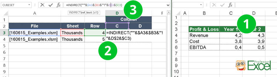
Let’s take a closer look at how to build the formula. The INDIRECT formula has only one argument: The link to another cell which can also be located within another workbook.
- Copy the first source cell.
- Paste it into your main file using paste special (Ctrl + Alt + v ). Instead of pasting it normally, click on “Link” in the bottom left corner of the Paste Special window. That way, you extract the complete path. In our case, we have the following link:
=[160615_Examples.xlsm]Thousands!$C$4 - Now we wrap the INDIRECT formula around this path. Furthermore, we separate it into file name, sheet name and cell reference. That way, we can later on just change one of these references, for instance for different versions of the same file. The complete formula looks like this (please also see the image above):
=INDIRECT(“‘”&$A3&$B3&”‘!”&D$2&$C3)
Important – please note: This function only works if the source workbooks are open.
Method 4: Merge files with a simple VBA macro
You are not afraid of using a simple VBA macro? Then let’s insert a new VBA module:
- Go to the Developer ribbon. If you can’t see the Developer ribbon, right click on any ribbon and then click on “Customize the Ribbon…”. On the right hand side, set the tick at “Developer”.
- Click on Visual Basic on the left side of the Developer ribbon.
- Right click on your workbook name and click on Insert –> Module.
- Copy and paste the following code into the new VBA module. Position the cursor within the code and click start (the green triangle) on the top. That’s it!
Sub mergeFiles()
    'Merges all files in a folder to a main file.

    'Define variables:
    Dim numberOfFilesChosen, i As Integer
    Dim tempFileDialog As fileDialog
    Dim mainWorkbook, sourceWorkbook As Workbook
    Dim tempWorkSheet As Worksheet

    Set mainWorkbook = Application.ActiveWorkbook
    Set tempFileDialog = Application.fileDialog(msoFileDialogFilePicker)

    'Allow the user to select multiple workbooks
    tempFileDialog.AllowMultiSelect = True

    numberOfFilesChosen = tempFileDialog.Show

    'Loop through all selected workbooks
    For i = 1 To tempFileDialog.SelectedItems.Count

        'Open each workbook
        Workbooks.Open tempFileDialog.SelectedItems(i)

        Set sourceWorkbook = ActiveWorkbook

        'Copy each worksheet to the end of the main workbook
        For Each tempWorkSheet In sourceWorkbook.Worksheets
            tempWorkSheet.Copy after:=mainWorkbook.Sheets(mainWorkbook.Worksheets.Count)
        Next tempWorkSheet

        'Close the source workbook
        sourceWorkbook.Close
    Next i

End Sub
Method 5: Automatically merge workbooks
The fifth way is probably most convenient:
Click on “Merge Files” on the Professor Excel ribbon.
Now select all the files and worksheets you want to merge and start with “OK”.
This procedure works well also for many files at the same time and is self-explanatory. Even better: Besides XLSX files, you can also combine XLS, XLSB, XLSM, CSV, TXT and ODS files.
To do that you need a third party add-in, for example our popular “Professor Excel Tools” (click here to start the download).
Here is the whole process in detail:
Method 6: Use the Get & Transform tools (PowerQuery)
The current version of Excel 365 offers the “Get & Transform” tools to import data. These functions are very powerful and are supposed to replace the old “Text Import Wizard”. However, they have one useful feature: Import a complete folder of documents.
The requirements: The workbooks and worksheets you want to import have to be in the same format.
Please follow these steps for importing a complete folder of Excel files.
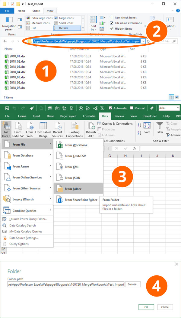
- Create a folder with all the documents you want to import.
- Usually it’s the fastest to just copy the folder path directly from the Windows Explorer. You still have the change to later-on select the folder, though.
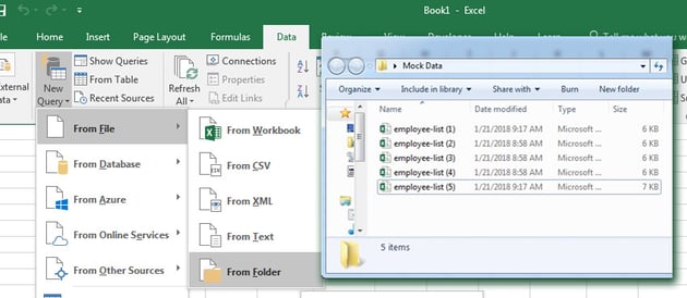
- Within Excel, go to the Data ribbon and click on “Get Data”, “From File” and then on “From Folder”.
- Paste the previously copied path or select it via the “Browse” function. Continue with “OK”.
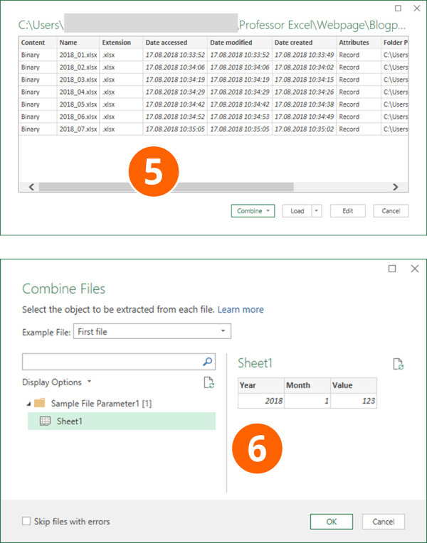
- If all files are shown in the following window, either click on “Combine” (and then on “Combine & Load To”) or on “Edit”. If you click on “Edit”, you can still filter the list and only import a selection of the files in the list. Recommendation: Put only the necessary files into your import folder from the beginning so that you don’t have to navigate through the complex “Edit” process.
- Next, Excel shows an example of the data based on the first file. If everything seems fine, click on OK. If your files have several sheets, just select the one you want to import, in this example “Sheet1”. Click on “OK”.
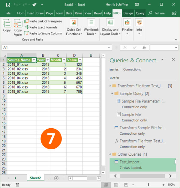
- That’s it, Excel now imports the data and inserts a new column containing the file name.
For more information about the Get & Transform tools please refer to this article.
Next step: Merge multiple worksheets to one combined sheet
After you have combined many Excel workbooks into one file, usually the next step is this: Merge all the imported sheets into one worksheet.
Because this is a whole different topic by itself, please refer to this article.
Image by MartinHolzer from Pixabay
If you’re a Microsoft Excel user, it doesn’t take long before you have many different workbooks full of important spreadsheets. What happens when you need to combine these multiple workbooks together so that all of the sheets are in the same place?
Excel can be challenging at times because it’s so powerful. You know that what you want to do is possible, but you might not know how to accomplish it. In this tutorial, I’ll show you several techniques you can use to merge Excel spreadsheets.
When you need to combine multiple spreadsheets, don’t copy and paste the data from each sheet manually. There are many shortcuts that you can use to save time in combining workbooks, and I’ll show you which one is right for each situation.


Watch & Learn
The screencast below will show you how to combine Excel sheets into a single consolidated workbook. I’ll teach you to use PowerQuery (also called Get & Transform Data) to pull together data from multiple workbooks.
Important: The email addresses used in this tutorial are fictitious (randomly generated) and not intended to represent any real email addresses.
Read on to see written instructions. As always, Excel has multiple ways to accomplish this task, and how you’re working with your data will drive which approach is the best.
1. How to Move & Copy Sheets (Simplest Method)
The easiest method to merge Excel spreadsheets is to simply take the entire sheet and copy it from one workbook to another.
To do this, start off by opening both Excel workbooks. Then, switch to the workbook that you want to copy several sheets from.
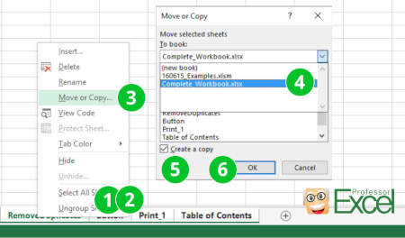
Now, hold Control (or Command on Mac) on your keyboard and click on all of the sheets that you want to copy to a separate workbook. You’ll notice that as you do this, the tabs will show as highlighted.
Now, simply right click and choose Move or Copy from the menu.


On the Move or Copy pop up window, the first thing that you’ll want to do is select the workbook that you want to move the sheets to. Choose the name of the file from the «To book» drop-down.


Also, you can choose where the sheets are placed in the new workbook in terms of sequence. The Before sheet menu controls where sequentially in the workbook the sheets will be inserted. You can always choose (move to end) and re-sequence the order the sheets later as needed.
Finally, it’s optional check the box to Create a copy, which will duplicate the sheets and create a separate copy of them in the workbook you’re moving the sheets to. Once you press OK, you’ll see that the sheets we copied are in the combined workbook.


This approach has a few downsides. If you keep working with two separate files, they aren’t «in sync.» If you make changes to the original workbook that you copied the sheets from, they won’t automatically update in the combined workbook.
2. Prepare to Use Get & Transform Data Tools to Combine Sheets
Excel has an incredibly powerful set of tools that are often called PowerQuery. Beginning with Excel 2016, this feature set was rebranded as Get & Transform Data.
As the name suggests, these are a set of tools that helps you pull data together from other workbooks and consolidate it into one workbook.


Also, this feature is exclusive to Excel for Windows. You won’t find it in the Mac versions or in the web browser edition of Microsoft’s app.
Before You Start: Check the Data
The most important part of this process is checking your data before you start combining it. The files need to have the same setup for the data structure, with the same columns. You can’t easily combine a four-column spreadsheet and a five-column spreadsheet, as Excel won’t know where to place the data.


Often, you’ll find yourself needing to combine spreadsheets when you’re downloading data from systems. In that case, it’s much easier to make sure the system you’re downloading data is configured to download data in the same columns each time.
Before I download data from a service like Google Analytics, I always make sure that I’m downloading the same report format each time. This ensures that I can easily work with and combine multiple spreadsheets together.
Whether you’re pulling data from a system like Google Analytics, MailChimp, or an ERP like SAP or Oracle that powers huge companies, the best way to save time is to ensure that you’re downloading data in a common format.
Now that we’ve checked our data, it’s time to dive into learning how to combine Excel sheets.
3. How to Combine Excel Sheets in a Folder Full of Files
A few times, I’ve had a folder full of files that I needed to put together into a single, consolidated file. When you’ve got dozens or even hundreds of files, opening them one-by-one to combine them just isn’t feasible. Learning this technique can save you dozens of hours on a single project.
Again, it’s crucial that the data is in the same format. To get started, it helps to place all of the files in the same folder so that Excel can easily watch this folder for changes.


Step 1. Point Excel to the Folder of Files
On the pop-up window, you’ll want to specify a path to the folder that holds your Excel workbooks.


You can browse to that path, or simply paste in the path to the folder with your workbooks.
Step 2. Confirm the List of Files
After you show Excel where the workbooks are stored, a new window will pop up that shows the list of files you’re set to combine. Right now, you’re only seeing metadata about the files, and not the data inside of it.


This window simply shows the files that are going to be combined with our query. You’ll see the file name, the type, and the dates accessed and modified. If you’re missing a file in this list, confirm that all of the files are in the folder and retry the process.
To move on to the next step, click on Edit.
Step 3. Confirm the Combination
The next menu helps to confirm the data inside your files. Since we’ve already checked that data is the same structure in our multiple files, we can simply click OK on this step.


Step 4. How to Combine Excel Sheets With a Click
Now, a new window pops up with the list of files we’re set to combine.
At this stage, you’re still seeing metadata about the files and now the data itself. To solve that, click on the double drop-down arrow in the upper right corner of the first column.


Voila! Now, you’ll see the actual data from inside the files combined into one place.


Scroll through the data to confirm that all of your rows are there. Notice that the only change from your original data is that the filename of each source file is in the first column.
Step 5. Close and Load the Data
Believe it or not, we’re basically finished with combining our Excel spreadsheets. The data is in the Query Editor for now, so we’ll need to «send it back» to regular Excel so that we can work with it.
Click on Close & Load in the upper right corner. You’ll see the finished data in a regular Excel spreadsheet, ready to review and work with.


Imagine using this feature to roll up multiple files from different members of your team. Choose a folder that you’ll each store files in, and then combine them into one cohesive file with this feature in just a few minutes.
Recap & Keep Learning
In this tutorial, you learned several techniques for how to combine Excel sheets. When you’ve got many sheets that you need to stitch together, using one of these approaches will save you time so that you can get back to the task at hand!
Check out some of the other tutorials to level up your Excel skills. Each of these tutorials will teach you a method for accomplishing tasks in less time in Microsoft Excel.
How do you merge Excel workbooks? Let me know in the comments section below whether you’ve got a preference for these methods, or a technique of your own that you use.
Did you find this post useful?

I believe that life is too short to do just one thing. In college, I studied Accounting and Finance but continue to scratch my creative itch with my work for Envato Tuts+ and other clients. By day, I enjoy my career in corporate finance, using data and analysis to make decisions.
I cover a variety of topics for Tuts+, including photo editing software like Adobe Lightroom, PowerPoint, Keynote, and more. What I enjoy most is teaching people to use software to solve everyday problems, excel in their career, and complete work efficiently. Feel free to reach out to me on my website.
Merging multiple sheets into one worksheet is a tough task, but thankfully we have a feature called “Consolidate” in Excel. Excel 2010 onwards, we can use “Power Query” as a worksheet merger. This article will show you how to merge worksheets into one.
Table of contents
- Merge Worksheet in Excel
- Merger Worksheet Using Consolidate Option
- Merge Worksheets by Using Power Query
- Things to Remember
- Recommended Articles
Getting the data in multiple worksheets is common but combining all the worksheet data at once is the job of the person who receives the data in different sheets.
Merger Worksheet Using Consolidate Option
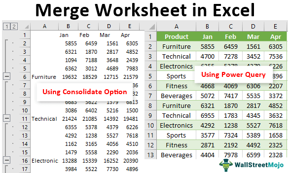
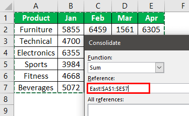
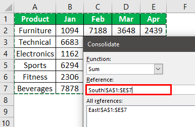
The easiest and quickest way to merge multiple worksheets data into one is by using the in-built feature of excel “Consolidate.” For example, look at the below data in Excel sheets.
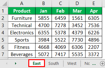
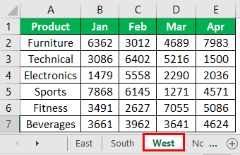
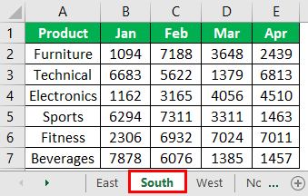
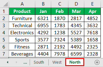
The above image has four worksheets comprising four different regions’ product-wise sales numbers across months.
We need to create one single sheet from the four above to show all the summary results. Then, follow the below steps to consolidate worksheets.
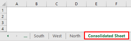
Step 1: We must first create a new worksheet and name it a “Consolidated Sheet.“
Step 2: We must now place a cursor in the first cell of the worksheet.
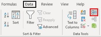
- Then, go to the “Data” tab.
- Click on the “Consolidate” option.
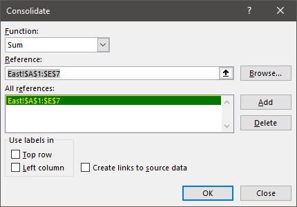
Step 3: As a result, this will open up below the “Consolidate” window.
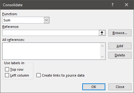
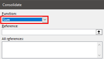
Step 4: Since we are consolidating all the four region data, choose the option of “Sum” under the function drop-down list in excelA drop-down list in excel is a pre-defined list of inputs that allows users to select an option.read more.
Step 5: Next, we need to choose the reference range from the first sheet to the last sheet. Place the cursor inside the reference box, go to the “East” sheet, and choose the data.
Step 6: Click on the “Add” button to add the first reference area.
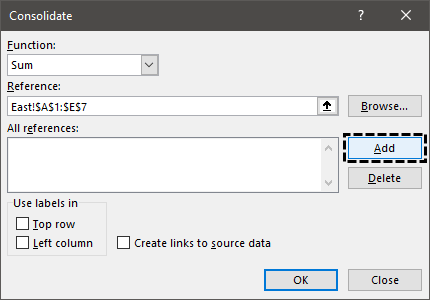
Now, this is added to the reference list.
Step 7: Next, we have to go to the “South” sheet, and the reference range would have been selected automatically.
Step 8: Click on “Add” again, and the second sheet reference is added to the list. Like this, we can repeat the same for all the sheets.
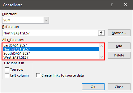
Now, we have added all four sheets of references. One more thing, while selecting each selected region range, including the row headerExcel Row Header is the grey column on the left side of column 1 in the worksheet that contains the numbers (1, 2, 3, etc.). To hide or reveal row and column headers, press ALT + W + V + H.read more and column header of the data table, to bring the same into the consolidated sheet, we must check the boxes of “Top Row” and “Left Column” and “Create links to Source Data.”
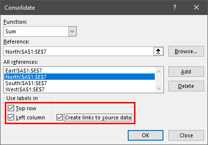
Click on “OK.” We will have a summary table like the one below.
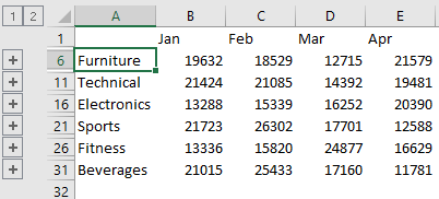
As we can see above, we have two grouped sheets, 1 and 2. If we click on 1, it will show all the region’s consolidated table, and if we click on 2, it will show the breakup of each zone.

It looks fine, but this is not the merging of worksheets. So, merging is combining all the worksheets into one without any calculations; we need to use the “Power Query” option.
Merge Worksheets by Using Power Query
The “Power Query” option is an add-in for ExcelAn add-in is an extension that adds more features and options to the existing Microsoft Excel.read more 2010 and 2013 versions. It is a built-in feature for Excel 2016 onwards versions.
Follow the steps to merge worksheets using Excel’s “Power Query” option.
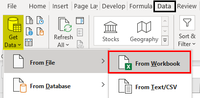
- We must go to the “Data” tab. Then, from the “Get Data,” select “From File,” “From Workbook.”

- Then, we must select the sheet and then transform it into a Power Query Editor.
We need to convert all the data tables into Excel tables. We have converted each data table into an Excel table and named East, South, West, and North by their region names.
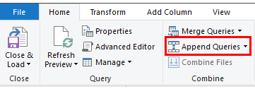
- First, we must go to any of the sheets. Then, under the “Power Query,” click on “Append Queries.”

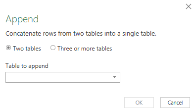
- Now, this will open up the “Append” window.

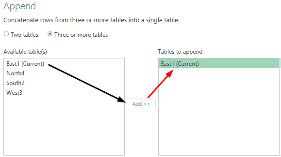
- Here, we need to merge more than one table, so we must choose the “Three or more tables” option.

- Then, select the table “East 1 (Current)” and click on the “Add” button.

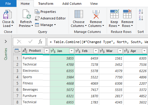
For other region tables, we need to repeat the same steps. - After this, click on “OK,” and it will open the “Power Query Editor” window.

- Finally, we must click on the “Close and Load” option.

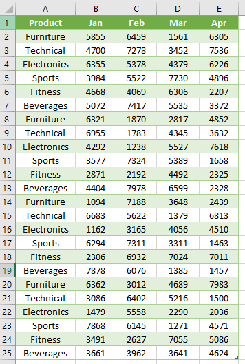
Consequently, this will merge all the sheets into one in a new worksheet of the same workbook.

Things to Remember
- The Power Query in excelPower Query is an excel tool used to import data from different sources, transform (change) it as required, and return a refined dataset in the workbook.read more is available for Excel 2010 and 2013 versions as an “Add-in.” From Excel 2016 onwards, this is a built-in tab.
- We can use the “Consolidate” option to consolidate different worksheets into one sheet based on arithmetic calculations.
- We need to convert the data into excel table formatExcel comes with a number of table styles that you may quickly apply to a table format. In Excel, you can design and use a new custom table style of your choice. read more for the “Power Query” merge.
Recommended Articles
This article has been a guide to Excel Worksheet Merge. Here, we discuss merging worksheets into one using the “Consolidate” and “Power Query” options and practical examples. You may learn more about Excel from the following articles: –
- Power Query Tutorial
- Column Merge Excel
- Examples of Combine Cells in Excel
- Merge Tables Excel
- Unmerge Cells Excel
Содержание
- Combine data from multiple sheets
- Combine by position
- Combine by category
- Combine by position
- Combine by category
- merge excel files
- 5 answers
- Merge Sheets: Easily Copy Excel Sheets Underneath on One Sheet!
- Method 1: Copy and paste worksheets manually
- Method 2: Use the INDIRECT formula to merge sheets
- Approach
- Download
- Method 3: Merge sheets with a VBA Macro
- Method 4: Combine sheets with “Professor Excel Tools”
- (New) Method 5: Merge sheets using the Office clipboard
Combine data from multiple sheets
If you receive information in multiple sheets or workbooks that you want to summarize, the Consolidate command can help you pull data together onto one sheet. For example, if you have a sheet of expense figures from each of your regional offices, you might use a consolidation to roll up these figures into a corporate expense sheet. That sheet might contain sales totals and averages, current inventory levels, and highest selling products for the whole enterprise.
To decide which type of consolidation to use, look at the sheets you are combining. If the sheets have data in inconsistent positions, even if their row and column labels are not identical, consolidate by position. If the sheets use the same row and column labels for their categories, even if the data is not in consistent positions, consolidate by category.
Combine by position
For consolidation by position to work, the range of data on each source sheet must be in list format, without blank rows or blank columns in the list.
Open each source sheet and make sure that your data is in the same position on each sheet.
In your destination sheet, click the upper-left cell of the area where you want the consolidated data to appear.
Note: Make sure that you leave enough cells to the right and underneath for your consolidated data.
On the Data tab, in the Data Tools group, click Consolidate.

In the Function box, click the function that you want Excel to use to consolidate the data.
In each source sheet, select your data.
The file path is entered in All references.
When you have added the data from each source sheet and workbook, click OK.
Combine by category
For consolidation by category to work, the range of data on each source sheet must be in list format, without blank rows or blank columns in the list. Also the categories must be consistently labeled. For example, if one column is labeled Avg. and another is labeled Average, the Consolidate command will not sum the two columns together.
Open each source sheet.
In your destination sheet, click the upper-left cell of the area where you want the consolidated data to appear.
Note: Make sure that you leave enough cells to the right and underneath for your consolidated data.
On the Data tab, in the Data Tools group, click Consolidate.
In the Function box, click the function that you want Excel to use to consolidate the data.
To indicate where the labels are located in the source ranges, select the check boxes under Use labels in: either the Top row, the Left column, or both.
In each source sheet, select your data. Make sure to include either the top row or left column information that you previously selected.
The file path is entered in All references.
When you have added the data from each source sheet and workbook, click OK.
Note: Any labels that don’t match labels in the other source areas cause separate rows or columns in the consolidation.
Combine by position
For consolidation by position to work, the range of data on each source sheet must be in list format, without blank rows or blank columns in the list.
Open each source sheet and make sure that your data is in the same position on each sheet.
In your destination sheet, click the upper-left cell of the area where you want the consolidated data to appear.
Note: Make sure that you leave enough cells to the right and underneath for your consolidated data.
On the Data tab, under Tools, click Consolidate.
In the Function box, click the function that you want Excel to use to consolidate the data.
In each source sheet, select your data, and then click Add.
The file path is entered in All references.
When you have added the data from each source sheet and workbook, click OK.
Combine by category
For consolidation by category to work, the range of data on each source sheet must be in list format, without blank rows or blank columns in the list. Also the categories must be consistently labeled. For example, if one column is labeled Avg. and another is labeled Average, the Consolidate command will not sum the two columns together.
Open each source sheet.
In your destination sheet, click the upper-left cell of the area where you want the consolidated data to appear.
Note: Make sure that you leave enough cells to the right and underneath for your consolidated data.
On the Data tab, under Tools, click Consolidate.
In the Function box, click the function that you want Excel to use to consolidate the data.
To indicate where the labels are located in the source ranges, select the check boxes under Use labels in: either the Top row, the Left column, or both.
In each source sheet, select your data. Make sure to include either the top row or left column information that you previously selected, and then click Add.
The file path is entered in All references.
When you have added the data from each source sheet and workbook, click OK.
Note: Any labels that don’t match labels in the other source areas cause separate rows or columns in the consolidation.
Источник
merge excel files

How to merge several Excel file into one worksheet in Excel?
5 answers
To merge several Excel files into one worksheet in Excel, you can use the following steps:
- Open the first Excel file that you want to merge.
- Go to the worksheet that you want to merge the other files into.
- Click the cell where you want to start the merge.
- Go to the Data tab and click on the “From Other Sources” button in the “Get External Data” group.
- Choose “From Microsoft Query” and click OK.
- In the Choose Data Source dialog box, select the “Microsoft Excel” option and click OK.
- In the Select Workbook dialog box, navigate to the location of the second Excel file that you want to merge and select it.
- Choose the worksheet in the second Excel file that you want to merge, and click OK.
- Repeat the process for each additional Excel file that you want to merge, selecting the appropriate worksheet from each file.
- When you’re finished, click the “Return Data” button to bring the data into your first worksheet.
- You may need to adjust the formatting of the merged data to make it look the way you want.
These steps will merge the data from several Excel files into one worksheet in a new workbook. You can save this workbook as a new file, or copy and paste the merged data into an existing workbook.
Power Query is the best way to merge or combine data from multiple Excel files in a single file. You need to store all the files in a single folder and then use that folder to load data from those files into the power query editor. It also allows you to transform that data along with combining it.
It works something like this:
- Saving All the Files into a Single Folder
- Combining them using Power Query
- Merging Data into a Single Table
- Make sure to download these sample file from here to follow along and check out this tutorial to learn power query.
Note: For combining data from different Excel files, your data should be structured in the same way. That means the number of columns and their order should be the same.
To merge files, you can use the following steps:
- First of all, extract all the files from the sample folder and save that folder at the desktop (or wherever you want to save it).
- Now, the next thing is to open a new Excel workbook and open “POWER Query”.
- For this, go to Data Tab вћњ Get & Transform Data вћњ Get Data вћњ From File вћњ From Folder.
- Here you need to locate the folder where you have files.
- In the end, click OK, and once you click OK, you’ll get a window listing all the file from the folder, just like below.
- Now, you need to combine data from these files and for this click on “Combine & Edit”.
- From here, the next thing is to select the table in which you have data in all the workbooks and yes, you’ll get a preview of this at the side of the window.
- Once you select the table, click OK. At this point, you have merged data from all the files into your power query editor and, if you look closely you can see a new column with the name of the workbooks from which data is extracted.
- So, right-click on the column header and select “Replace Values”.
- Here in the “Value to Replace” enter the text “.xlsx” and leave “Replace With” blank (here idea is to remove the file extension from the name of the workbook).
- After that, double click on the header and select “Rename” to enter a name for the column i.e. Zone
- At this point, your merged data is ready and all you need is to load it into your new workbook. So, go to the Home Tab and click on the “Close & Load”.
Now you have your combined data (from all the workbooks) into a single workbook.
This is the moment of JOY, write “Joy” in the comment section if you love to use “Power Query for combining data from multiple files”.
Источник
Merge Sheets: Easily Copy Excel Sheets Underneath on One Sheet!

Let’s assume you have many worksheets, all in the same structure. Or they are at least in a similar structure. Now, you want to combine them into one worksheet. For example copying them underneath each other so that you can conduct lookups or insert PivotTables. In this article, you learn four methods to merge sheets in Excel.
Method 1: Copy and paste worksheets manually
In many cases it’s probably the fastest way to just copy and paste each sheet separately. That depends of course on the number of worksheets you want to combine and their structure. Some comments:
- Try to use keyboard shortcuts as much as possible. For example for selecting the complete worksheet (Ctrl + A), copying the data (Ctrl + C), navigating to your combined worksheet (Ctrl + Page Up or Page Down) and pasting the copied cells (Ctrl + V).
- Also the shortcut of pressing Ctrl on the keyboard and clicking on the little arrow in the left bottom corner of your worksheet could help. That way you jump to the first or last worksheet in your Excel workbook.
- This method is especially useful if you just have to merge sheets once. If you need to do it repeatedly (for example you get new inputs every week or month) it’s probably better to check out methods 2 to 4 below.
Method 2: Use the INDIRECT formula to merge sheets
You can use Excel formulas to combine data from all worksheets. The main formula is INDIRECT.
This method has some disadvantages, though.
- The INDIRECT formula in general is slow because it’s volatile. That means, it calculates each time Excel calculates something.
- Using a combination of INDIRECT is usually unstable and error prone.
- It takes some work to set up the INDIRECT formula.
On the other hand, it has one major advantage: If you spend effort to set it up, this method is dynamic. That means when your input updates, the merged worksheet updates as well.
Approach
The INDIRECT formula can access any cell from a link (or better: an address) you provide. Please refer to this article to learn more about the INDIRECT formula. So you only have to provide the addresses for each cell in each worksheet you want to combine. Therefore, you should prepare a worksheet the following way (please refer to the screenshot on the right-hand side):
- Column A contains the sheet name.
- Column B contains the row number.
- Starting from Column C, you should add the column letters.
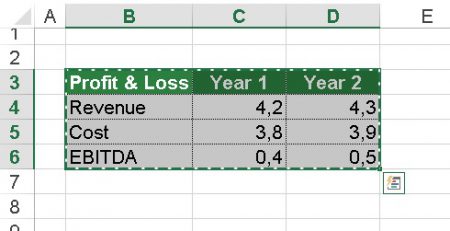
So let’s assume that you want to get the value from cell A1 of Sheet1. You would need then all the parts ‘Sheet1’, column ‘A’ and row ‘1’. Combining them in the INDIRECT formula would lead to the following formula. The formula in cell C4 is =INDIRECT(“‘”&$A4&”‘!”&C$2&$B4) .
Download

You want to save some time? We prepared a worksheet which can merge sheets automatically. What do you have to do? Download this workbook (
7 MB) and copy the only sheet into your own workbook. That’s it.
Please note the following comments.
- This method requires to enable macros (a list of all worksheets in your workbook is automatically created). When you want to save your workbook, you will be asked to switch to the XSLM file format.
- This model works for up to 50 sheets with 200 rows each (10,000 cells are prepared). If you need more, you have to extend it. The reason for this restriction is that the file is already quite large and requires some calculation performance.
Method 3: Merge sheets with a VBA Macro
You feel confident enough to use a simple VBA macro? Please insert the following code into a new VBA module. If you need assistance with VBA, please refer to this article.
Method 4: Combine sheets with “Professor Excel Tools”
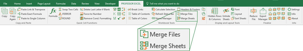
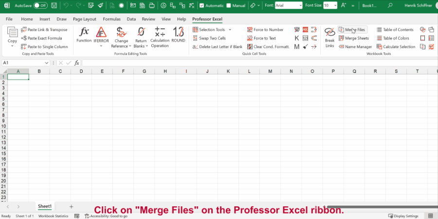
You like to use the most convenient way? Try the Excel add-in Professor Excel Tools.
- Just select all the worksheets you’d like to merge,
- click the button “Merge Sheets” and
- click on “Start”.
Alternatively, you can further refine your desired settings: Do you want to add the original sheet name in column A? No problem.
Also, define the copy & paste mode as shown in the screenshot on the right-hand side.

This function is included in our Excel Add-In ‘Professor Excel Tools’
(No sign-up, download starts directly)
More than 35,000 users can’t be wrong.
(New) Method 5: Merge sheets using the Office clipboard
The first method above already dealt with copying and pasting sheets manually. There is one more trick here: Use the Excel clipboard to merge sheets. It’s actually quite simple, just follow these steps.
- Open the clipboard: Click on the small arrow in the right bottom corner of the Clipboard section (on the Home ribbon).
- Now you can see the clipboard.
- Next, go through each worksheet. Copy all ranges which you later want to merge on one worksheet.
- Now, you can see all your copied ranges in the clipboard.
- Go to the sheet where you want to paste them underneath each other. Select the first cell.
- Click on “Paste all”
That’s it. Especially with larger files, this method could save some time compared to method number 1 above. One small disadvantage: You can further adjust the pasting method, for example using paste special to paste values only.
Источник