What is logical function in excel - Word и Excel - помощь в работе с программами

Excel for Microsoft 365 Excel for Microsoft 365 for Mac Excel for the web Excel 2021 Excel 2021 for Mac Excel 2019 Excel 2019 for Mac Excel 2016 Excel 2016 for Mac Excel 2013 Excel 2010 Excel 2007 Excel for Mac 2011 Excel Starter 2010 More…Less

To get detailed information about a function, click its name in the first column.

Note: Version markers indicate the version of Excel a function was introduced. These functions aren’t available in earlier versions. For example, a version marker of 2013 indicates that this function is available in Excel 2013 and all later versions.

Function	Description
AND function	Returns TRUE if all of its arguments are TRUE
BYCOL function	Applies a LAMBDA to each column and returns an array of the results
BYROW function	Applies a LAMBDA to each row and returns an array of the results
FALSE function	Returns the logical value FALSE
IF function	Specifies a logical test to perform
IFERROR function	Returns a value you specify if a formula evaluates to an error; otherwise, returns the result of the formula
IFNA function	Returns the value you specify if the expression resolves to #N/A, otherwise returns the result of the expression
IFS function	Checks whether one or more conditions are met and returns a value that corresponds to the first TRUE condition.
LAMBDA function	Create custom, reusable functions and call them by a friendly name
LET function	Assigns names to calculation results
MAKEARRAY function	Returns a calculated array of a specified row and column size, by applying a LAMBDA
MAP function	Returns an array formed by mapping each value in the array(s) to a new value by applying a LAMBDA to create a new value
NOT function	Reverses the logic of its argument
OR function	Returns TRUE if any argument is TRUE
REDUCE function	Reduces an array to an accumulated value by applying a LAMBDA to each value and returning the total value in the accumulator
SCAN function	Scans an array by applying a LAMBDA to each value and returns an array that has each intermediate value
SWITCH function	Evaluates an expression against a list of values and returns the result corresponding to the first matching value. If there is no match, an optional default value may be returned.
TRUE function	Returns the logical value TRUE
XOR function	Returns a logical exclusive OR of all arguments

Important: The calculated results of formulas and some Excel worksheet functions may differ slightly between a Windows PC using x86 or x86-64 architecture and a Windows RT PC using ARM architecture. Learn more about the differences.

Argument name	Description
logical_test (required)	The condition you want to test.

What is logical function example?

A logical test is used in logical functions to evaluate the contents of a cell location. The results of the logical test can be either true or false. For example, the logical test C7 = 25 (read as “if the value in cell C7 is equal to 25”) can be either true or false depending on the value that is entered into cell C7.

What is the main logical function in Excel?

IF function
The IF function is the main logical function in Excel and is, therefore, the one to understand first. It will appear numerous times throughout this article. Let’s have a look at the structure of the IF function, and then see some examples of its use. logical_test: This is the condition for the function to check.

How do you write an IF THEN statement?

Another way to define a conditional statement is to say, “If this happens, then that will happen.” The hypothesis is the first, or “if,” part of a conditional statement. The conclusion is the second, or “then,” part of a conditional statement. The conclusion is the result of a hypothesis.

Is VLOOKUP a logical function?

VLOOKUP is a powerful function to perform lookup in Excel. It performs a row-wise lookup until a match is found. The IF function performs a logical test and returns one value for a TRUE result, and another for a FALSE result.

What are logical functions in Excel 2010?

Excel 2010 uses seven logical functions — AND, FALSE, IF, IFERROR, NOT, OR, and TRUE — which appear on the Logical command button’s drop-down menu on the Formulas tab of the Ribbon. All the logical functions return either the logical TRUE or logical FALSE when their functions are evaluated.

What is logical function?

Logical functions are used in spreadsheets to test whether a situation is true or false. Depending on the result of that test, you can then elect to do one thing or another. These decisions can be used to display information, perform different calculations, or to perform further tests.

How do I use an IF function in Excel?

When you combine each one of them with an IF statement, they read like this:

AND – =IF(AND(Something is True, Something else is True), Value if True, Value if False)
OR – =IF(OR(Something is True, Something else is True), Value if True, Value if False)
NOT – =IF(NOT(Something is True), Value if True, Value if False)

How do you do multiple logic in Excel?

It is possible to nest multiple IF functions within one Excel formula. You can nest up to 7 IF functions to create a complex IF THEN ELSE statement. TIP: If you have Excel 2016, try the new IFS function instead of nesting multiple IF functions.

How is a logical test used in an IF formula?

The IF function runs a logical test and returns one value for a TRUE result, and another for a FALSE result. For example, to “pass” scores above 70: =IF(A1>70,”Pass”,”Fail”).The IF function can be combined with logical functions like AND and OR to extend the logical test.

How do you write an IF and then formula in Excel?

The syntax of IF-THEN is =IF(logic test,value if true,value if false). The first argument tells the function what to do if the comparison is true. The second argument tells the function what to do if the comparison is false.

Can you nest VLOOKUPs?

The VLOOKUP function will throw an #N/A error when a value isn’t found. By nesting multiple VLOOKUPs inside the IFERROR function, the formula allows for sequential lookups. If the first VLOOKUP fails, IFERROR catches the error and runs another VLOOKUP.

What is ISNA?

The ISNA function is a type of error handling function in Excel. It helps to find out whether any cell has “#N/A error” or not. This function returns the value “true” if “#N/A error” is identified. It returns “false” if there is any value other than “#N/A error.”

What is an Xlookup in Excel?

Use the XLOOKUP function to find things in a table or range by row.With XLOOKUP, you can look in one column for a search term, and return a result from the same row in another column, regardless of which side the return column is on.

What is logical calculation?

Logical calculations allow you to determine if a certain condition is true or false (boolean logic). For example, you might want to quickly see if sales for each country you distribute your merchandise to were above or below a certain threshold.

Can IF statement have 2 conditions?

Use two if statements if both if statement conditions could be true at the same time. In this example, both conditions can be true. You can pass and do great at the same time. Use an if/else statement if the two conditions are mutually exclusive meaning if one condition is true the other condition must be false.

How do I write a conditional formula in Excel?

You can create a formula-based conditional formatting rule in four easy steps:

Select the cells you want to format.
Create a conditional formatting rule, and select the Formula option.
Enter a formula that returns TRUE or FALSE.
Set formatting options and save the rule.

What are the 3 arguments of the IF function?

There are 3 parts (arguments) to the IF function:

TEST something, such as the value in a cell.
Specify what should happen if the test result is TRUE.
Specify what should happen if the test result is FALSE.

How does a VLOOKUP work?

The VLOOKUP function performs a vertical lookup by searching for a value in the first column of a table and returning the value in the same row in the index_number position.As a worksheet function, the VLOOKUP function can be entered as part of a formula in a cell of a worksheet.

How do I do a VLOOKUP with two criteria?

VLOOKUP with Multiple Criteria – Using a Helper Column

Insert a Helper Column between column B and C.
Use the following formula in the helper column:=A2&”|”&B2.
Use the following formula in G3 =VLOOKUP($F3&”|”&G$2,$C$2:$D$19,2,0)
Copy for all the cells.

How many IF functions can be nested in Excel?

While Excel will allow you to nest up to 64 different IF functions, it’s not at all advisable to do so.

Источник

Things will not always be the way we want them to be. The unexpected can happen. For example, let’s say you have to divide numbers. Trying to divide any number by zero (0) gives an error. Logical functions come in handy such cases. In this tutorial, we are going to cover the following topics.

In this tutorial, we are going to cover the following topics.

What is a Logical Function?
IF function example
Excel Logic functions explained
Nested IF functions

What is a Logical Function?

It is a feature that allows us to introduce decision-making when executing formulas and functions. Functions are used to;

Check if a condition is true or false
Combine multiple conditions together

What is a condition and why does it matter?

A condition is an expression that either evaluates to true or false. The expression could be a function that determines if the value entered in a cell is of numeric or text data type, if a value is greater than, equal to or less than a specified value, etc.

IF Function example

We will work with the home supplies budget from this tutorial. We will use the IF function to determine if an item is expensive or not. We will assume that items with a value greater than 6,000 are expensive. Those that are less than 6,000 are less expensive. The following image shows us the dataset that we will work with.

Put the cursor focus in cell F4
Enter the following formula that uses the IF function

=IF(E4<6000,”Yes”,”No”)

HERE,

“=IF(…)” calls the IF functions
“E4<6000” is the condition that the IF function evaluates. It checks the value of cell address E4 (subtotal) is less than 6,000
“Yes” this is the value that the function will display if the value of E4 is less than 6,000
“No” this is the value that the function will display if the value of E4 is greater than 6,000

When you are done press the enter key

You will get the following results

Excel Logic functions explained

The following table shows all of the logical functions in Excel

S/N	FUNCTION	CATEGORY	DESCRIPTION	USAGE
01	AND	Logical	Checks multiple conditions and returns true if they all the conditions evaluate to true.	=AND(1 > 0,ISNUMBER(1)) The above function returns TRUE because both Condition is True.
02	FALSE	Logical	Returns the logical value FALSE. It is used to compare the results of a condition or function that either returns true or false	FALSE()
03	IF	Logical	Verifies whether a condition is met or not. If the condition is met, it returns true. If the condition is not met, it returns false. =IF(logical_test,[value_if_true],[value_if_false])	=IF(ISNUMBER(22),”Yes”, “No”) 22 is Number so that it return Yes.
04	IFERROR	Logical	Returns the expression value if no error occurs. If an error occurs, it returns the error value	=IFERROR(5/0,”Divide by zero error”)
05	IFNA	Logical	Returns value if #N/A error does not occur. If #N/A error occurs, it returns NA value. #N/A error means a value if not available to a formula or function.	=IFNA(D6*E6,0) N.B the above formula returns zero if both or either D6 or E6 is/are empty
06	NOT	Logical	Returns true if the condition is false and returns false if condition is true	=NOT(ISTEXT(0)) N.B. the above function returns true. This is because ISTEXT(0) returns false and NOT function converts false to TRUE
07	OR	Logical	Used when evaluating multiple conditions. Returns true if any or all of the conditions are true. Returns false if all of the conditions are false	=OR(D8=”admin”,E8=”cashier”) N.B. the above function returns true if either or both D8 and E8 admin or cashier
08	TRUE	Logical	Returns the logical value TRUE. It is used to compare the results of a condition or function that either returns true or false	TRUE()

A nested IF function is an IF function within another IF function. Nested if statements come in handy when we have to work with more than two conditions. Let’s say we want to develop a simple program that checks the day of the week. If the day is Saturday we want to display “party well”, if it’s Sunday we want to display “time to rest”, and if it’s any day from Monday to Friday we want to display, remember to complete your to do list.

A nested if function can help us to implement the above example. The following flowchart shows how the nested IF function will be implemented.

The formula for the above flowchart is as follows

=IF(B1=”Sunday”,”time to rest”,IF(B1=”Saturday”,”party well”,”to do list”))

HERE,

“=IF(….)” is the main if function
“=IF(…,IF(….))” the second IF function is the nested one. It provides further evaluation if the main IF function returned false.

Practical example

Create a new workbook and enter the data as shown below

Enter the following formula

=IF(B1=”Sunday”,”time to rest”,IF(B1=”Saturday”,”party well”,”to do list”))

Enter Saturday in cell address B1
You will get the following results

Download the Excel file used in Tutorial

Summary

Logical functions are used to introduce decision-making when evaluating formulas and functions in Excel.

Источник

Logic Functions in Excel check the data and return the result «TRUE» if the condition is true, and «FALSE» if not.

Consider the syntax of logic functions and examples of their application in the process of working with the Excel program.

Logical functions in Excel and examples of solving the problems

Objective 1. It is necessary to overestimate the trade balances. If he product is kept in stock for more than 8 months we should reduce its price 2 times.

We form a table with initial parameters:

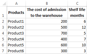
To solve the problem, use the logical IF function. The formula will have a look like this: =IF(C2>=8;B2/2;B2)

Logical expression «C2>=8» is constructed using relational operators «>» and «=». The result of his calculations is a logical value of «TRUE» or «FALSE». In the first case, the function returns the value «B2/2». In the second it’s «B2».

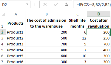
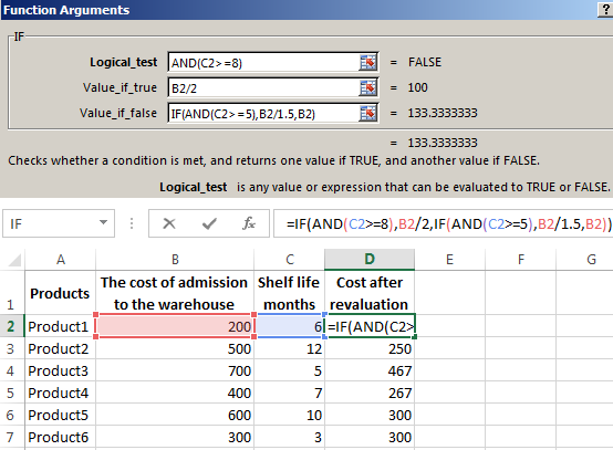
Let’s complicate the task — to employ the logic function И. Now we have such a condition: if the product is stored for more than 8 months, the price is reduced 2 times. If it’s more than 5 months, but less than 8, it’s 1.5 times.

The formula takes the following form:

IF.

The use of logic functions in Excel:

Function Name	Value	Syntax	Note
TRUE	It does not have arguments, it returns the logical value » TRUE «	TRUE	It is rarely used as an independent function
FALSE	It does not have arguments, it returns the logical value » FALSE «	FALSE	——-//——-
AND	If all the given arguments return true result, then the function issues a logical expression » TRUE «. If one of the function outputs the result «false» the whole function gives the result «FALSE»	=AND(boolean1;boolean2;…)	Accepts up to 255 arguments in the form of conditions or links. It is mandatory to first.
OR	It displays the result “TRUE“ if at least one of the arguments is true.	=OR(boolean1;boolean2;…)	——-//——-
NOT	It changes the logic value “TRUE on the contrary — » FALSE «. And vice versa.	#NAME?	Usually it is combined with other operators.
IF	Test the validity of a logical expression and returns the result	=IF (boolean;value_if_TRUE;value_if_FALSE)	« boolean » in the calculations should have results “ TRUE “ or “ FALSE “
IFERROR	If the first argument is true, it returns its argument. Otherwise it’s the value of the second argument.	= IFERROR(value;”error”)	Both arguments are mandatory.

The function IF can be used as arguments to the text values

Objective 2. If the value of the goods in the warehouse after the write-down was less than 300 r. or the product is stored for longer than 10 months, it is written off.

For the solution use logic functions IF and OR:

Condition recorded using a logical OR operation, stands as follows: goods are deducted if the number in cell D2 = 10.

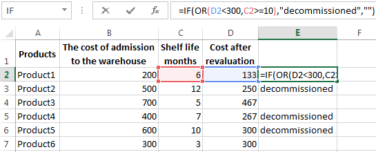
In terms of non-compliance with the conditions, IF function returns to an empty cell.

As arguments, you can use other functions. These are mathematical, for example.

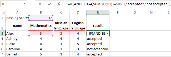
Objective 3. Students before entering the gymnasium pass math, English and Russian. Passing Score is 12. You should get at least 4 points in mathematics for admission. Create report on the receipt.

We set up a table with the source data:

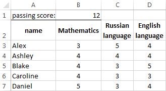
It is necessary to compare the total number of points with a passing grade. And check that math score was not lower than «4». In the «result» column put «accepted» or «not accepted».

There’s such a formula:

Logical operator «AND» causes the function to check the validity of the two conditions. The mathematical function «SUM» is used to calculate the final score.

AND.

The function IF allows us to solve many problems; it is therefore used more often.

The statistical and logical functions in Excel

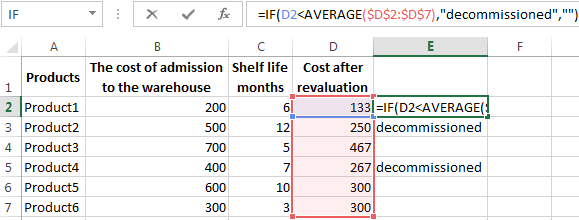
Task 1. Analyze the cost of cash balances after the devaluation. If the price of the product after reassessment is below average values, we should write off the product from the warehouse.

Working with the table in the previous section:

To solve the problem use the formula of such a form:

In logical terms «D2<AVERAGE (D2:D7)» apply statistical function AVERAGE. It returns the average of the range D2: D7.

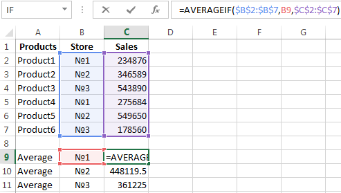
Task 2. Find the average sales in stores.

We set up a table with the source data:

table.

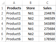
You need to find the arithmetic meaning for the cells, which value corresponds to a predetermined condition. That is to combine logical and statistical solution.

Below a table with a condition there’s the table to display the results.

We solve the problem with a single function:

The first argument $B$2:$B$7 is a range of cells for testing. The second argument B9 is a condition. The third argument the $C$2:$C$7 is an averaging range; the numerical values, which are taken to calculate the arithmetic mean.

AVERAGEIF function compares the value of B9 cells (№1) with values in the range B2: B7. That is the number of stores in the sales table. For matching the data considers the arithmetic mean of using numbers in the range C2: C7.

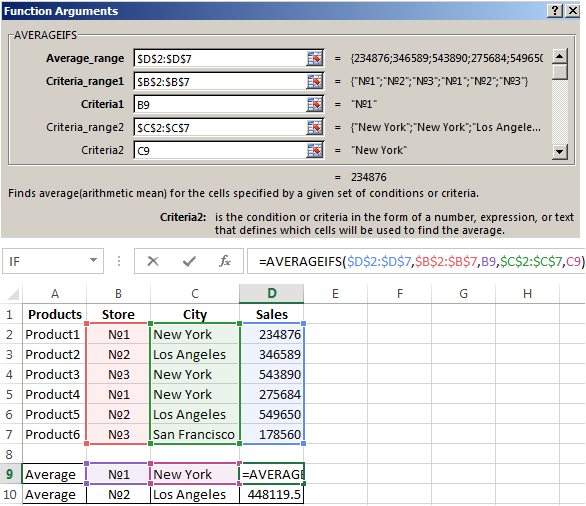
Task 3. Find the average sales in the store №1 New York and №2 Los Angeles.

Modify the table from the previous example:

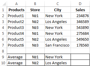
It is necessary to fulfill two conditions — use the function of the form:

Done.

Download examples logical functions

The function AVERAGEIFS allows you to use more than one condition. The first argument $D$2:$D$7 is an averaging ranges (where are the numbers to find the arithmetic mean). The second argument $B$2:$B$7 is a range to test the first condition. The third argument B9 is the first condition. The fourth and fifth arguments are the ranges for checking the second condition respectively.

The function takes into account only the values that meet all these criteria.

Источник

Excel Logical Functions (Table of Contents)

Introduction to Logical Functions in Excel
Types of Logical Functions in Excel

Introduction to Logical Functions in Excel

Logical functions in Excel work with conditions. They help deal with different situations accordingly. These functions perform work similar to IF-ELSEIF-ELSE statements in a programming language. All of these functions have simple syntaxes, and they can be beautifully combined with other functions to obtain desired results. There are various types of logical functions, some of which are commonly used in data operations in Excel.

Types of Logical Functions in Excel

The various types of logical functions in Excel are IF, IFERROR, AND, OR, NOT, TRUE, and FALSE. In the following section, we will see how to use each of them through examples.

You can download this Logical Functions Excel Template here – Logical Functions Excel Template

1. IF

It is a very simple logical function that checks if the condition to be validated as true or false. We will demonstrate the use of the IF function using a very simple example. There’s a simple dataset containing data of students and their marks. Now, if the passing marks are 40, then we would like to declare the result for each student in terms of PASS and FAIL. This can be done using the IF function.

Syntax:

Example:

Step 1: When we enter the IF function, Excel automatically pops up the list of arguments, as shown in the following screenshot.

Step 2: The first argument is the logical test. In this case, the condition is that if marks are more than 40, then the result is PASS, or else it is FAIL. We passed the condition as the argument in the IF function as shown below.

Step 3: The second and third arguments are ‘value_if_true’ and ‘value_if_false’, respectively. If marks are greater than 40, then the result should be PASS; otherwise, FAIL. This has been accomplished by passing the arguments as shown in the following screenshot.

Step 4: Copy the IF function across all the required cells, and we are returned the correct result as shown in the following screenshot.

2. IFERROR

This function is used when we want to return some meaningful result in place of an error. There are various types of errors in Excel, and IFERROR is used to deal with these errors. At many times, in Excel, we are returned error values as results. In such cases, the IFERROR function becomes handy.

Syntax:

As we can see in the syntax, the IFERROR function basically means that if the value passed into it is not an error value, then that value will be given as output by the function; otherwise, the value that we have specified in ‘value if error’ argument.

Step 1: The IFERROR function takes into consideration two arguments as seen in the syntax. This is also shown in the screenshot below.

Step 2: In this example, we have marks for certain students. For some of the students, the result is not available, and for them, we have a #N/A error in the Marks column. We want this error value to be replaced with some meaningful text which is possible through the use of IFERROR. The following screenshot shows this.

As we can see in the above screenshot, we passed marks as the first argument and kept the string “Not Available” as the second argument. It means if marks are valid, then output marks or else “Not Available”. This is as shown by the following screenshot.

3. AND

This function returns either TRUE or FALSE value by checking the conditions that are passed into it. If all the conditions passed into AND function are met, then the TRUE value is returned, and if even a single condition is not met, then the FALSE value is returned.

Syntax:

Step 1: We have marks for three different subjects for certain students. Now, we want to check if the student has passed or failed. If a student secures marks less than 40 even in a single subject out of the three subjects, he has failed in the examination. We can determine the result for each student using the AND function. When we enter the AND function, we find that arguments are highlighted. In this case, they are logical conditions, as shown below.

Step 2: Using AND, we will get results for each student by passing the conditions in the function as shown below.

When the function is implemented, we get the result as shown below. Note, here, TRUE means pass, and FALSE means fail.

4. OR

It returns TRUE value even if a single condition out of the total conditions passed into it is met. It returns FALSE when all the arguments are FALSE.

Syntax:

Step 1: We have marks for three different subjects for certain students. Now, if a student has secured 40 marks in at least one of the three subjects, then the result should be pass or else fail. When we enter the OR function, the arguments are highlighted as below.

Step 2: The desired criteria for determining a student’s result can be met using the OR function as shown below.

When the above step is followed, we get the desired result, as shown below. Observe it.

5. NOT

It reverses the logical value, i.e. TRUE to FALSE and FALSE to TRUE. It is implemented usually in context-based situations.

Syntax: NOT(logical)

Step 1: We pass certain logical conditions into NOT and check how the function works. Have a look at the following screenshot.

The actual result for each of them is shown. However, the logical values are reversed when we pass the logical conditions into the NOT function, as shown below.

6. TRUE and FALSE

They return corresponding logical values; TRUE returns TRUE while FALSE returns FALSE.

Syntax: TRUE(), FALSE()

We have the result of students. For PASS, we will display TRUE and for FAIL, FALSE. The following screenshot shows the implementation.

The result that we obtain is as shown below.

Things to Remember

The logical functions should be implemented in various contexts to understand their full capability.
The difference in available features in logical functions for different versions of Excel should be checked.
Each of the argument in a logical function should be studied in order to understand its role and significance.

List of Logical Functions

Let’s go over the list of logical functions that are available in excel and learn how we can use them in our day-to-day work.

1. AND function

AND function is one of the logical functions in Excel, which determines whether all criteria in a test are TRUE. it returns TRUE if all of its parameters are TRUE, and FALSE if one or more arguments are FALSE.

Syntax: AND(logical1, [logical2], …), where logical1 is the first condition you want to test is one that can be TRUE or FALSE and logical2… are optional and additional conditions up to a maximum of 255 conditions.

The following example shows the use of AND function:

Select the cell where you want to display the result.
Type =AND(A1>50,B1<50) where cells A1 and B1 contain numeric values.

Press the Enter key to display the result.

2. FALSE function

The FALSE function in Excel returns the logical FALSE value.

Syntax: FALSE(), it has no arguments. Microsoft Excel will read the word FALSE without parentheses as the logical value FALSE if you write it directly onto the worksheet or into a formula.

3. IF function

One of Excel’s most used tools is the IF function, which allows you to create logical comparisons. An IF statement can have two possible outcomes. If the comparison is TRUE, the first result is returned; if the comparison is FALSE, the second result is returned.

Syntax: IF(logical_test,value_if_true,[value_if_false]), where logical_test is the comparison you want to test, value_if_true is the value to be returned if the logical_test is TRUE, and value_if_false is the value to b returned if the logical_test is FALSE. The following example shows the use of the IF function:

Select the cell where you want to display the result.
Type =IF(A1>B1,”A1>B1″,”A1<B1″) where cells A1 and B1 contain numeric values.

Press the Enter key to display the result.

4. IFERROR function

The IFERROR function can be used to catch and manage errors in a formula. If a formula evaluates to an error, IFERROR returns a value you specify; otherwise, it returns the formula’s result.

Syntax: IFERROR(value, value_if_error), where value is the condition to be checked for #N/A, #VALUE!, #REF!, #DIV/0!, #NUM!, #NAME?, or #NULL! error and value_error is the custom message to be returned if the formula evaluates to an error. The following example shows the use of the IFERROR function:

Select the cell where you wan to display the result.
Type =IFERROR(A2/B2,”Error in calculation”) where cells A2 and B2 contain the dividend and divisor respectively.

Press the Enter key to display the result. As, you can see the divisor is zero, so a #DIV/0! should be returned. IFERROR fucntion catches the error and returns the custom message.

5. IFS function

The IFS function determines whether one or more criteria are met and returns the value corresponding to the first TRUE condition. With several criteria, IFS can replace nested IF statements and is considerably easier to read.

Syntax: IFS(logical_test1, value_if_true1, [logical_test2, value_if_true2], [logical_test3, value_if_true3],…), where logical_test1 is the first comparison you want to test, value_if_true 1 is the value to be returned if the logical_test1 is TRUE and the same follows for other conditions. The following example shows the use of IFS function:

Select the cell where you want to display the result.
Type =IFS(A2>89,”A”,A2>79,”B”,A2>69,”C”,A2>59,”D”,A2<=59,”F”) to assign letter grades on the basis of marks obtained.

Press the Enter key to display the result. The value returned is “B” as 85>79 and 85<90.

6. NOT function

The NOT function returns the inverse of its argument’s value. It is frequently used to extend the utility of other functions that perform logical tests.

Syntax: NOT(logical), where logical is a value or expression that may be tested to determine whether it is TRUE or FALSE. The following example shows the use of the NOT function:

Select the cell where you want to display the result.
Type =NOT(TRUE), to reverse TRUE value to FALSE.

Press the Enter key to display the result.

7. OR function

The OR function returns TRUE if any of its parameters are TRUE and FALSE if all of its arguments are FALSE.

Syntax: OR(logical1, [logical2], …), where logical1, logical2, logical3 etc, are conditions to be evaluated for TRUE and FALSE values. The following example shows the use of the OR function:

Select the cell where you want to display the result.
Type =OR(A1<50,B1>50) where cells A1 and B1 contain numeric values.

Press the Enter key to display the result.

8. SWITCH function

The SWITCH function compares one value called the expression to a list of values and returns the first matched value as the result. If no match is found, a default value is returned.

Syntax: SWITCH(expression, value1, result1, [default or value2, result2],…[default or value3, results]), where expression is the value to be compared, value1… are the values to compare an expression to, and result1… are the results to be returned corresponding to the matching value of the expression. The following example shows the use of the SWITCH function:

Select the cell where you want to display the result.
Type =SWITCH(A2,1,”Gold”,2,”Silver”,3,”Bronze”) to decide medals on the basis of rank in cell A2.

Press the Enter key to display the result.

9. TRUE function

The TRUE function in Excel returns the logical TRUE value.

Syntax: TRUE(), it has no arguments. Microsoft Excel will read the word TRUE without parentheses as the logical value TRUE if you write it directly onto the worksheet or into a formula.

10. XOR function

The XOR function returns a TRUE value when the number of true inputs is odd otherwise it returns FALSE. Syntax: XOR(logical1, [logical2],…), where logical1, logical2, logical3 etc, are conditions to be evaluated for TRUE or FALSE values. The following example shows the use of XOR function:

Select the cell where you want to display the result.
Type =XOR(A1>50,B1<50,C1<25) where cells A1, B1 and C1 contain numeric values.

Press the Enter key to display the result. The XOR fucntion returns FALSE value as 2 conditions are TRUE and 2 is an even number.

Conclusion

In this article, we learned about the various logical functions in Excel.

References

AND function (microsoft.com)
FALSE function (microsoft.com)
IF function (microsoft.com)
IFERROR function (microsoft.com)
IFS function (microsoft.com)
NOT function (microsoft.com)
OR function (microsoft.com)
SWITCH function (microsoft.com)
TRUE function (microsoft.com)
XOR function (microsoft.com)

Источник

Logical functions in Excel are functions that test whether a specified condition is true or false. The result of the logical test will determine whether to evaluate or not to evaluate a function. For example, based on the result of the test, we can evaluate a function, display information, or display TRUE or FALSE.

There are several logical functions in excel, but the most used are the AND, OR, NOT, and XOR functions. In this tutorial, we are going to explore how to use the AND, OR, NOT, and XOR logical functions in Excel.

What are logical functions in Excel?

When there is a need to make a decision before evaluating data in Excel, logical functions will be employed. Logical functions in Excel are decision-making tools used to analyze excel data. When it is employed, it tests a cell and returns a value based on the correct decision.

The AND, OR, NOT, and XOR logical functions return a TRUE or FALSE value depending on the decision evaluated. To evaluate a function and return a value, these functions are used alongside the IF function.

For example, the formula: =IF(AND(C3=”South”,D3=”Uche Golden”),”Correct”,”Wrong”) will return CORRECT or WRONG depending on the values of C3 and D3. In this tutorial, we shall discuss how to use the four logical functions displayed in the table below.

Function	Detail	Example	Remark
AND	Evaluates to TRUE if all arguments are true	=AND(C3=”South”,D3=”Uche Golden”)	Returns TRUE only if C3 is South and D3 is Uche Golden
OR	Evaluates to TRUE if any of the arguments are true	=OR(C3=”South”,D3=”Uche Golden”)	Returns TRUE if C3 is South or D3 is Uche Golden or one of them is true or both of them are true.
NOT	Evaluates to TRUE if the argument is false, and vice versa	=NOT(C3=“South”)	Returns TRUE only if C3 is not South. I.e. if C3 is West, it returns TRUE.
XOR	Evaluates to TRUE only if the argument is an exclusive OR	=XOR(C3=”South”,D3=”Uche Golden”)	Returns TRUE if C3 is South and D3, not Uche Golden, or if C3 if not South and D3 are Uche Golden.

Facts about logical functions in excel

When using the logical functions in Excel, you should attempt to observe the following important facts.

Microsoft Excel 2003 version and lower accepts up to 30 arguments of a logical function. However, the formula length shall not exceed 1024 characters.
Microsoft Excel 2007 and higher accepts up to 255 arguments of a logical function. But the formula length shall not exceed 8192 characters.
Logical functions accept any of the following arguments: Mcrosoft Excel functions, numbers, texts, cell references, Booleans, and comparison operators.
Logical functions do not evaluate a value but return a Boolean value of TRUE or FALSE.

Using the AND, OR, NOT, and XOR Functions in Excel

The AND, OR, NOT and XOR statements return a TRUE or FALSE value depending on the result of the logical test. They use the following arguments:

AND [=AND(logical1,logical2,logical3,…)] – A TRUE is returned if all the logical values are true else FALSE is returned.

OR [=OR(logical1,logical2,…)] – A TRUE is returned if one or both of the logical values are true else FALSE is returned

NOT [=NOT(Logical)] – A TRUE is returned if the logical value is true else FALSE is returned. A logical value is true when the value is not present in the referenced cell.

XOR [=XOR(logical1,logical2,…)] – A TRUE is returned if one of the logical values are true else FALSE is returned.

AND function in Excel

The AND function compares more than one condition in the function’s argument. It returns TRUE only if all conditions in the argument are met, and false, if otherwise. This means that when three conditions are specified, the AND returns TRUE if all three conditions are true. If one of the conditions is not true, the AND function returns FALSE.

Let us assume two conditions, A and B in an argument, the AND TRUE table is as follow: =AND(A2=“A”, B2=“B”)

Condition A	Condition B	AND Value
A is true	B is true	TRUE
A is true	B is false	FALSE
A is false	B is true	FALSE
A is false	B is false	FALSE

The syntax of the AND function is given as follow:

=AND(logical1, [logical2],…)

Where AND is the Microsoft Excel function to be evaluated
Logical1 is a required argument that must be specified. It is the condition that will be tested and it evaluates to either TRUE or FALSE.
[logical2] is anoptional argument. When specified, it increases the chances of the argument evaluating to FALSE.
The optional argument can be increased to up to 254 if the length of the formula is below 8192. Hence, you can have logical3, logical 4, … logicaln.

The AND function in Excel Example

The table below displays the departments and salaries of different staff of a named organization. Using the AND function, identify the staff in the clerk department whose salary is below 10000.

To solve the above problem, do the following:

Enter the required data in Excel as shown in the worksheet above.
Create a column called “Clerks that earn 10000 and below”
Enter the formula in cell D2, =AND(C2=”Clerk”,B2<=10000)
Use the autofill handle to fill the formula to other cells below D2.
The result of the function is displayed below

The function displays TRUE if both conditions, “Clerk” and <=10000 are true, and false if otherwise. You can use the AND function to identify ADMIN staff who earns above 10000.

OR function in Excel

The OR function also compares more than one condition in the function’s argument. It returns TRUE if any of the conditions in the argument are met. It, however, returns FALSE if none of the conditions are met.

This implies that when three conditions are specified, the OR function returns TRUE if any or all three conditions are true. If none of the conditions is true, the OR function returns FALSE.

Let us assume two conditions, A and B in an argument, the OR TRUE table is as follow: =OR(A2=“A”, B2=“B”)

Condition A	Condition B	OR Value
A is true	B is true	TRUE
A is true	B is false	TRUE
A is false	B is true	TRUE
A is false	B is false	FALSE

The OR logical function in Excel returns false only when none of the arguments is true.

The syntax of the OR function is given as follow:

=OR(logical1, [logical2],…)

Where OR is the Excel function to be evaluated
Logical1 is a required argument that must be specified. It is the condition that will be tested and it evaluates to either TRUE or FALSE.
[logical2] is anoptional argument. When specified, it increases the chances of the argument evaluating to TRUE.
The optional argument can be increased to up to 254 if the length of the formula is below 8192. Hence, you can have logical3, logical 4, … logicaln.

The OR function in Excel Example

The table below displays the departments and salaries of different staff of a named organization. Using the OR function, identify the staff in the Admin department or those who earn above 10000.

To solve the above problem, do the following:

Use the same data you used in the AND function example
Create a new column called “Admin Staff and those who earn above 10000”
Enter the formula in cell E2, =OR(B2>10000,C2=”Admin”)
Use the autofill handle to fill the formula to other cells below E2.

The result of the function displays TRUE if any of the conditions are true. Here, if staff is in ADMIN, OR evaluates as TRUE, if the salary is >10000, OR evaluates as TRUE. Also, if staff is admin and salary above 10000, OR evaluates as TRUE. But if staff is not ADMIN, and salary is not above 10000, OR evaluates to FALSE.

NOT function in Excel

The NOT function is used to exclude the values you do not want in a function. It returns the opposite of the logical condition in the function’s argument. For example, if the logical test is TRUE, the NOT function returns a FALSE value and vice versa.

The NOT function has only one argument which can be a text, cell reference, etc. Any value in the argument is excluded when the function is evaluated. For example, =NOT(A2=“Blue”) means every other color except blue.

The NOT TRUE table is as follow: =NOT(A2=“A”)

Condition A	OR Value
A is true	FALSE
A is false	TRUE

The NOT logical function in Excel returns false only when the argument in the function is true.

The syntax of the NOT function is given as follow:

=NOT(logical)

Where NOT is the Excel function to be evaluated
logical is a required argument that must be specified. It is the condition that will be tested and it evaluates to either TRUE or FALSE.

The NOT function in Excel Example

The table below displays the departments and salaries of different staff of a named organization. Using the NOT function, identify the staff that is not in the Accounts department.

To solve the above problem, do the following:

Use the same data you used in the AND function example
Create a new column called “Staff not in ACT Dept.”
Enter the formula in cell F2, =NOT(C2=”Act”)
Use the autofill handle to fill the formula to other cells below F2.

The result of the function displays TRUE if the condition is false, and FALSE if the condition is true. Here, if staff is in Admin, Clerk, or Messenger, NOT evaluates as TRUE, if staff is in ACT, NOT evaluates to FALSE.

XOR function in Excel

This is called the exclusive OR function. The XOR function is used to compare more than one condition in the function’s argument. It returns TRUE if any of the conditions in the argument is met. It, however, returns FALSE if both or none of the conditions are met.

This implies that when three conditions are specified, the XOR function returns TRUE if any of all three conditions are true. If none or all of the conditions are true, the XOR function returns FALSE.

Let us assume two conditions, A and B in an argument, the XOR TRUE table is as follow: =XOR(A2=“A”, B2=“B”)

Condition A	Condition B	OR Value
A is true	B is true	FALSE
A is true	B is false	TRUE
A is false	B is true	TRUE
A is false	B is false	FALSE

The XOR logical function in Excel returns false only when all or none of the arguments is true.

The syntax of the XOR function is given as follow:

=XOR(logical1, [logical2],…)

Where XOR is the Excel function to be evaluated
Logical1 is a required argument that must be specified. It is the condition that will be tested and it evaluates to either TRUE or FALSE.
[logical2] is anoptional argument. The optional argument can be increased to up to 254 if the length of the formula is below 8192. Hence, you can have logical3, logical 4, … logicaln.

The XOR function in Excel Example

The table below displays the departments and salaries of different staff of a named organization. Identify those who are exclusively in the Mess department or earns less than 10000.

Let’s use the XOR function to identify those in the Mess dept. or those who earn below 10000.

Use the same data you used in the AND function example
Create a new column called “Mess Staff or those who earn below 10000”
Enter this formula in cell G2, =XOR(B2<10000,C2=”Mess”)
Use the autofill handle to fill the formula to other cells below G2.

The result of the function displays TRUE if any of the conditions are true. Here, if staff is in Mess and salary 10000 and above, XOR evaluates as TRUE. If salary is <10000 and staff not in Mess dept., XOR evaluates as TRUE. But, if staff is in Mess and salary below 10000, XOR evaluates as FALSE. Also, if staff is not in Mess and salary above 10000, XOR evaluates to FALSE.

Conclusion

Logical functions in Excel are used to test the conditions of an argument whether it is TRUE or FALSE. There are different built-in logical functions in Excel, but the most used ones are AND, OR, NOT, and XOR.

Each of the logical functions evaluates to TRUE or FALSE. To return the actual value, the IF function will be employed.

The AND, OR, and XOR functions compare more than one condition while the NOT function excludes specified conditions.

It is important to master these functions because we shall use them with the IF Statement to return values. Before we continue with the IF Statement in Excel next week, remember to visit our previous tutorials. Don’t forget to share this tutorial with friends.

Источник

Содержание

Logical functions (reference)
IF function
Simple IF examples
Common problems
Need more help?
Logical functions in Excel with the examples of their use
Logical functions in Excel and examples of solving the problems
The use of logic functions in Excel:
The function IF can be used as arguments to the text values
The statistical and logical functions in Excel

Logical functions (reference)

To get detailed information about a function, click its name in the first column.

Note: Version markers indicate the version of Excel a function was introduced. These functions aren’t available in earlier versions. For example, a version marker of 2013 indicates that this function is available in Excel 2013 and all later versions.

Returns TRUE if all of its arguments are TRUE

BYCOL function

Applies a LAMBDA to each column and returns an array of the results

BYROW function

Applies a LAMBDA to each row and returns an array of the results

Returns the logical value FALSE

Specifies a logical test to perform

Returns a value you specify if a formula evaluates to an error; otherwise, returns the result of the formula

IFNA function

Returns the value you specify if the expression resolves to #N/A, otherwise returns the result of the expression

IFS function

Checks whether one or more conditions are met and returns a value that corresponds to the first TRUE condition.

LAMBDA function

Create custom, reusable functions and call them by a friendly name

LET function

Assigns names to calculation results

MAKEARRAY function

Returns a calculated array of a specified row and column size, by applying a LAMBDA

MAP function

Returns an array formed by mapping each value in the array(s) to a new value by applying a LAMBDA to create a new value

Reverses the logic of its argument

Returns TRUE if any argument is TRUE

REDUCE function

Reduces an array to an accumulated value by applying a LAMBDA to each value and returning the total value in the accumulator

SCAN function

Scans an array by applying a LAMBDA to each value and returns an array that has each intermediate value

SWITCH function

Evaluates an expression against a list of values and returns the result corresponding to the first matching value. If there is no match, an optional default value may be returned.

Returns the logical value TRUE

XOR function

Returns a logical exclusive OR of all arguments

Important: The calculated results of formulas and some Excel worksheet functions may differ slightly between a Windows PC using x86 or x86-64 architecture and a Windows RT PC using ARM architecture. Learn more about the differences.

Источник

IF function

The IF function is one of the most popular functions in Excel, and it allows you to make logical comparisons between a value and what you expect.

So an IF statement can have two results. The first result is if your comparison is True, the second if your comparison is False.

For example, =IF(C2=”Yes”,1,2) says IF(C2 = Yes, then return a 1, otherwise return a 2).

Use the IF function, one of the logical functions, to return one value if a condition is true and another value if it’s false.

IF(logical_test, value_if_true, [value_if_false])

The condition you want to test.

The value that you want returned if the result of logical_test is TRUE.

The value that you want returned if the result of logical_test is FALSE.

Simple IF examples

In the above example, cell D2 says: IF(C2 = Yes, then return a 1, otherwise return a 2)

In this example, the formula in cell D2 says: IF(C2 = 1, then return Yes, otherwise return No)As you see, the IF function can be used to evaluate both text and values. It can also be used to evaluate errors. You are not limited to only checking if one thing is equal to another and returning a single result, you can also use mathematical operators and perform additional calculations depending on your criteria. You can also nest multiple IF functions together in order to perform multiple comparisons.

B2,”Over Budget”,”Within Budget”)» loading=»lazy»>

=IF(C2>B2,”Over Budget”,”Within Budget”)

In the above example, the IF function in D2 is saying IF(C2 Is Greater Than B2, then return “Over Budget”, otherwise return “Within Budget”)

B2,C2-B2,»»)» loading=»lazy»>

In the above illustration, instead of returning a text result, we are going to return a mathematical calculation. So the formula in E2 is saying IF(Actual is Greater than Budgeted, then Subtract the Budgeted amount from the Actual amount, otherwise return nothing).

In this example, the formula in F7 is saying IF(E7 = “Yes”, then calculate the Total Amount in F5 * 8.25%, otherwise no Sales Tax is due so return 0)

Note: If you are going to use text in formulas, you need to wrap the text in quotes (e.g. “Text”). The only exception to that is using TRUE or FALSE, which Excel automatically understands.

Common problems

What went wrong

There was no argument for either value_if_true or value_if_False arguments. To see the right value returned, add argument text to the two arguments, or add TRUE or FALSE to the argument.

This usually means that the formula is misspelled.

Need more help?

You can always ask an expert in the Excel Tech Community or get support in the Answers community.

Источник

Logical functions in Excel with the examples of their use

Logic Functions in Excel check the data and return the result «TRUE» if the condition is true, and «FALSE» if not.

Consider the syntax of logic functions and examples of their application in the process of working with the Excel program.

Logical functions in Excel and examples of solving the problems

Objective 1. It is necessary to overestimate the trade balances. If he product is kept in stock for more than 8 months we should reduce its price 2 times.

We form a table with initial parameters:

To solve the problem, use the logical IF function. The formula will have a look like this: =IF(C2>=8;B2/2;B2)

The formula takes the following form:

=8),B2/2,IF(AND(C2>=5),B2/1.5,B2))’ >

The use of logic functions in Excel:

Function Name	Value	Syntax	Note
TRUE	It does not have arguments, it returns the logical value » TRUE «	TRUE	It is rarely used as an independent function
FALSE	It does not have arguments, it returns the logical value » FALSE «	FALSE	——-//——-
AND	If all the given arguments return true result, then the function issues a logical expression » TRUE «. If one of the function outputs the result «false» the whole function gives the result «FALSE»	=AND(boolean1;boolean2;…)	Accepts up to 255 arguments in the form of conditions or links. It is mandatory to first.
OR	It displays the result “TRUE“ if at least one of the arguments is true.	=OR(boolean1;boolean2;…)	——-//——-
NOT	It changes the logic value “TRUE on the contrary — » FALSE «. And vice versa.	#NAME?	Usually it is combined with other operators.
IF	Test the validity of a logical expression and returns the result	=IF (boolean;value_if_TRUE;value_if_FALSE)	« boolean » in the calculations should have results “ TRUE “ or “ FALSE “
IFERROR	If the first argument is true, it returns its argument. Otherwise it’s the value of the second argument.	= IFERROR(value;”error”)	Both arguments are mandatory.

The function IF can be used as arguments to the text values

For the solution use logic functions IF and OR:

Condition recorded using a logical OR operation, stands as follows: goods are deducted if the number in cell D2 = 10.

In terms of non-compliance with the conditions, IF function returns to an empty cell.

As arguments, you can use other functions. These are mathematical, for example.

Objective 3. Students before entering the gymnasium pass math, English and Russian. Passing Score is 12. You should get at least 4 points in mathematics for admission. Create report on the receipt.

We set up a table with the source data:

It is necessary to compare the total number of points with a passing grade. And check that math score was not lower than «4». In the «result» column put «accepted» or «not accepted».

There’s such a formula:

Logical operator «AND» causes the function to check the validity of the two conditions. The mathematical function «SUM» is used to calculate the final score.

The function IF allows us to solve many problems; it is therefore used more often.

The statistical and logical functions in Excel

Task 1. Analyze the cost of cash balances after the devaluation. If the price of the product after reassessment is below average values, we should write off the product from the warehouse.

Working with the table in the previous section:

To solve the problem use the formula of such a form:

Task 2. Find the average sales in stores.

We set up a table with the source data:

You need to find the arithmetic meaning for the cells, which value corresponds to a predetermined condition. That is to combine logical and statistical solution.

Below a table with a condition there’s the table to display the results.

We solve the problem with a single function:

Task 3. Find the average sales in the store №1 New York and №2 Los Angeles.

Modify the table from the previous example:

It is necessary to fulfill two conditions — use the function of the form:

The function takes into account only the values that meet all these criteria.

Источник

See Also

Need more help?

Want more options?

What is logical function example?

What is the main logical function in Excel?

How do you write an IF THEN statement?

Is VLOOKUP a logical function?

What are logical functions in Excel 2010?

What is logical function?

How do I use an IF function in Excel?

How do you do multiple logic in Excel?

How is a logical test used in an IF formula?

How do you write an IF and then formula in Excel?

Can you nest VLOOKUPs?

What is ISNA?

What is an Xlookup in Excel?

What is logical calculation?

Can IF statement have 2 conditions?

How do I write a conditional formula in Excel?

What are the 3 arguments of the IF function?

How does a VLOOKUP work?

How do I do a VLOOKUP with two criteria?

How many IF functions can be nested in Excel?

What is a Logical Function?

IF Function example

Excel Logic functions explained

Practical example

Summary

Logical functions in Excel and examples of solving the problems

The use of logic functions in Excel:

The function IF can be used as arguments to the text values

The statistical and logical functions in Excel

Introduction to Logical Functions in Excel

Types of Logical Functions in Excel

1. IF

2. IFERROR

3. AND

4. OR

5. NOT

6. TRUE and FALSE

Things to Remember

Recommended Articles

List of Logical Functions

1. AND function

2. FALSE function

3. IF function

4. IFERROR function

5. IFS function

6. NOT function

7. OR function

8. SWITCH function

9. TRUE function

10. XOR function

Conclusion

References

What are logical functions in Excel?

Facts about logical functions in excel

Using the AND, OR, NOT, and XOR Functions in Excel

AND function in Excel

The AND function in Excel Example

OR function in Excel

The OR function in Excel Example

NOT function in Excel

The NOT function in Excel Example

XOR function in Excel

The XOR function in Excel Example

Conclusion

Logical functions (reference)

IF function

Simple IF examples

Common problems

Need more help?

Logical functions in Excel with the examples of their use

Logical functions in Excel and examples of solving the problems

The use of logic functions in Excel:

The function IF can be used as arguments to the text values

The statistical and logical functions in Excel

А вот еще интересные статьи: